Solar activity prediction

CONCLUSION - Morphological.

The presence of sunspots on the Sun had been known long before the seventeenth century; however, it was Galileo Galilei who, around 1610, first treated them as a physically meaningful object of scientific study. Notably, this occurred shortly before the onset of the Maunder Minimum (~1645–1700). Nevertheless, it was only in the mid-nineteenth century that Heinrich Schwabe discovered the quasi-periodic nature of solar activity, and Rudolf Wolf introduced a quantitative measure—the sunspot number—thereby initiating systematic studies of solar cycles. A modern account of the development of solar activity research and the rise of dynamo theory is presented in the book Nature’s Third Cycle: A Story of Sunspots by A. R. Choudhuri.

When focusing primarily on sunspots (SSN), three main time series are currently available. The first is the classical sunspot number record, which provides high-detail observations but is relatively short in duration, beginning around 1700 [1]. The second is a long cosmogenic-isotope-based series spanning approximately 10,000 years with a temporal resolution comparable to the solar cycle, reconstructed by Sami Solanki et al. (2004). The third is another isotope-based series covering about one thousand years, in which 93 individual solar cycles have been identified, but without resolving individual Gleissberg cycles, as reported by Ilya Usoskin et al. (2025).

The fact that a structural approach can be implemented only through morphological analysis of the classical sunspot record is due to fundamental differences in the effective resolution of these datasets. In a broad sense, classical sunspot number records provide a high-resolution view of solar activity, preserving the morphology of individual cycles and allowing centennial-scale variability to appear as distinct Gleissberg cycles, whereas cosmogenic isotope records represent a low-resolution, integral proxy in which the same long-term variability manifests primarily as smooth modulation.

In this context, the introduction of structure should be regarded not merely as a descriptive refinement, but as an additional dimension in the understanding of solar activity. Beyond amplitudes, periods, and long-term modulation, the solar cycle reveals an internal organization that constrains the set of dynamically admissible states and governs transitions between them. From this perspective, centennial-scale variability does not simply modulate an otherwise repetitive process but reflects slow rearrangements in the coherent architecture of the system itself.

Within this broader framework, dynamo theory occupies a natural but limited position. In its classical form, the solar dynamo is commonly interpreted as a nonlinear auto-oscillator—a self-sustained regime arising from the interaction of differential rotation, magnetic induction, and feedback through the Lorentz force. Such auto-oscillatory behavior represents one of the simplest stable modes available to complex nonlinear systems, characterized by robustness, phase coherence, and insensitivity to moderate perturbations. While this interpretation successfully explains the existence and persistence of the 11-year cycle, it does not, by itself, exhaust the dynamical possibilities of the system.

More generally, nonlinear systems far from equilibrium are known to admit multiple organized regimes, whose emergence and stability are governed by principles of self-organization. As emphasized in the works of Ilya Prigogine, dissipative structures arise when fluxes and instabilities cooperate to produce order rather than disorder. In a complementary formulation, Hermann Haken introduced the concept of slaving, whereby a small number of macroscopic modes impose coherence on a large number of microscopic degrees of freedom.

Seen from this angle, the solar dynamo may be interpreted not as an isolated mechanism, but as an executive oscillatory regime embedded within a higher-level self-organized system. The observed structural regularities of solar activity—including the organization of cycles into centennial-scale patterns—can then be viewed as manifestations of coherent behavior emerging from the collective dynamics of the solar convection zone. In this sense, coherence is not imposed externally, nor encoded solely in the dynamo equations, but arises naturally from the system’s capacity to self-organize across multiple temporal and spatial scales. See for example: Krist ́of Petrovay,  “Solar cycle prediction”, arXiv:1907.02107v2 [astro-ph.SR] 4 Mar 2020. Dibyendu Nandy, "Progress in solar cycle predictions: sunspot cycles 24 - 25 in perspective", arXiv:2009.01908v1 [astro-ph.SR] 3 Sep 2020. Charbonneau, P. “Dynamo models of the solar cycle”. Living Rev Sol Phys 17, 4 (2020).

The Sun’s detailed morphology—including discrete H-pairs, slow MEC-waves, multi-level interconnections, structural form memory, and the implicit constraints that forbid configurations such as complete loss of H-pairs, disruption of MEC-waves, breakdown of inter-level coordination, or violation of H-pair parity—unequivocally characterizes its behavior as coherent and structurally organized. These morphological and dynamical features indicate that the Sun is far more than a stochastic or auto collective α–Ω dynamo: it is a hierarchically structured system with intrinsic constraints and memory, capable of preserving identity, structural integrity, and long-term stability across centennial timescales. Observed magnetic fields, cycle amplitudes, H-pair sequences, and long-term modulations emerge as manifestations of this underlying coherent architecture, rather than as independent drivers of solar dynamics, demonstrating that the apparent variability of solar activity is tightly constrained by an internally consistent set of allowable states. Thus, the Sun possesses a coherent architecture that preserves its dynamical stability over millennia.

The MEC - wave is not something extraordinary; it is merely a characteristic order parameter as in all complex dissipative systems, from the Universe to humans. Across these levels, four universal features of management emerge naturally:

1. Channeling energy flows: Energy itself is given, but management directs it into coherent patterns—gravity shapes cosmic structures, MCE organizes convective energy in the Sun, metabolism structures energy on Earth, and the psyche channels neural and hormonal activity.
2. Creating memory and history: Management preserves past states to influence future ones—galactic structures encode mass distributions, MCE cycles impose long-term solar patterns, life stores genetic and epigenetic information, and the mind preserves experiences shaping behavior.
3. Sustaining order amidst chaos: Management stabilizes systems against intrinsic fluctuations—turbulent cosmic and solar motions, ecological interactions, or emotional and cognitive noise are organized into enduring structures.
4. Hierarchy of scales and times: Local processes are embedded in broader frameworks—fast cosmic events, convective eddies, metabolic cycles, or instantaneous neural impulses all integrate into slower, larger-scale patterns.

In every case, energy provides potential, and management transforms it into structure, memory, and continuity, enabling the system to persist and evolve.

Concluding remarks. The MHD system of the solar convection zone (SCZ) is structured, but not rigidly so. Much depends on how the current S-cycle has developed. Its principal characteristics are To, Hm, PMF**m and ε.                  

For example, cycle #2 is the shortest (about 0.9 of the mean duration for short cycles), whereas cycle #4 is the longest (about 1.1 of the mean duration for long cycles).

Five discrete levels of Hm are observed, although with notable nuances (see the vertical arrows in Fig. 2B). Deviations of up to ±20%, and even anomalies (e.g., cycle #13), may occur, yet the overall structure remains preserved.

The parameter ε requires separate consideration. It can introduce a factor of order two, which is nevertheless regulated by the system’s structure: this applies to saddle-type single S-cycles, while the effect is more moderate for H-paired cycles. This difference reflects the fact that saddle S-cycles arise from relatively rare transitional bifurcations, whereas the more numerous paired S-cycles represent local regimes of the SCZ MHD system.

In essence, the present work is devoted exclusively to the morphological aspect of solar activity (in the adopted representation). Although the morphology of solar activity in our analysis is complete and self - consistent, its results remain physically unjustified.

As for the physical MHD theory of solar activity, it therefore appears to be incomplete, particularly with respect to structural organization. The emergence of H - paired S-cycles, the discreteness of parameters, the existence of nine types of MA-cycles, the fixation of the GL-cycle structure at its beginning and end, the fact that the GL-cycle always contains exactly four H-pairs, as well as the origin of BHF, all remain unexplained.

This points not to shortcomings of individual mechanisms, but to the absence of a connecting level of description—one in which morphology and MHD dynamics are coupled. Contemporary theory operates either with local processes of magnetic field generation and transport, or with averaged cycles, thereby losing the structural integrity of the phenomenon. As a result, the observed hierarchy of cycles is treated as an empirical fact rather than as a necessary consequence of the system’s dynamics.

This leads to a paradoxical situation: a morphological scheme lacking physical derivation proves to be more structurally definite than the physical theory intended to explain it. Resolving this contradiction would apparently require the introduction of an intermediate description, in which the large-scale evolution of flows in the convection zone acts not as a background, but as an active organizing factor of solar activity.

In its present form, the discrepancy between morphology and physics ceases to be a methodological subtlety and becomes a matter of principle. Either the observed structural organization of solar activity—including rigidly fixed cycle configurations and their hierarchy—is a secondary, statistically accidental superposition on MHD processes, or these processes themselves are described at a level insufficient to reproduce the actually existing organization. Both assumptions are equally unsatisfactory: the former contradicts the stability and reproducibility of the observed forms, while the latter calls into question the completeness of the physical theory. As long as this gap persists, solar activity remains a phenomenon that can be numerically modeled, but not, in the strict sense, understood.

General stellar structure theory, and in particular the theory of the solar interior, identify the solar convective zone (SCZ) as a complex dissipative MHD system, in which energy transported from the core through the radiative zone is converted into large-scale plasma motions and associated magnetic fields. The latter are indirectly observed at the photosphere, most notably in the form of sunspots. Rudolf Wolf proposed to quantify solar activity by sunspot counts, thereby introducing the sunspot number (SSN) time series. At present, SSN data exist in three principal forms, differing in temporal resolution and duration: daily data (D-data, since 1 January 1818), monthly data (M-data, since January 1749), and cosmogenic proxy records (C-data; e.g. ¹⁰Be and ¹⁴C isotopes), which have a temporal resolution of the order of the solar cycle but extend over millennia. I developed a morphology of solar activity based on the M-data series, which contains three Gleissberg-length (GL) cycles. Morphological analysis reveals a finite set of stable states and a strictly constrained structure of transitions between them. These empirical regularities impose nontrivial constraints that any physical model of the SCZ must satisfy. At this stage, they constitute a system of phenomenologically established facts whose underlying physical connections remain unexplained.  Since the SCZ is a dissipative MHD system and therefore capable of self-organization, its long-term evolution can be naturally described in terms of a structured phase space. We introduce the concept of Phase-Space Topology (PST) of the SCZ: a geometrically constrained organization of admissible trajectories that governs transitions between observable morphological states. In this framework, the empirically identified stable states correspond to dynamically preferred regions of phase space, while the observed transition rules reflect its topological structure. Standard dynamo approaches do not naturally reproduce such a constrained topology of transitions, which motivates the development of a morphology-driven solar dynamo (MDSD) theory formulated explicitly in PST terms. Within this approach, solar activity cycles are interpreted as trajectories evolving inside a slowly deforming phase-space topology, where morphological regularities emerge as macroscopic manifestations of underlying MHD dynamics. 

Summing up the first, most labor-intensive, and at the same time, the section containing the core new information on the structures of solar activity emerging in its SSN morphology, it should be noted that, as the work progressed, the question of the need for a convincing explanation of the obtained morphological results increasingly came to the fore. Solar activity and its principal phenomenon—the solar cycle—are a by-product of MHD processes developing in the SCZ, which is usually described as an infinite-dimensional system of PDEs and, in turn, constitutes a dissipative dynamical system potentially prone to structural self-organization. In this context, it is natural to turn to the theory of dissipative dynamical systems (DDST) for such an explanation. This theory studies the behavior of complex systems of various kinds using ODEs. It has long been recognized that, despite their complexity, such systems exhibit behavior that is, in practice, understandable. Time in these systems flows from the past to the future; the paths they follow (trajectories in phase space) converge onto a global attractor (A); and if it is possible to embed it into a smooth inertial manifold (IM), where trajectories are shaped by slow variables (sV), then the system’s established behavior can be described by ODEs, the solutions of which constitute a limit cycle evolving over time—that is, throughout the system’s evolution. This theory is powerful, though not simple, and a natural question arises: to what extent do our morphological results correspond to its fundamental concepts?

                                                                                                      Morphology and theory - are they compatible?

Solar activity, being a multifaceted phenomenon, is examined from various scientific perspectives. This website investigates the nature of its periodicity from morphological, dynamical, and physical viewpoints. The primary focus is on morphology (see above), and the results are interpreted through the lens of the theory of dissipative dynamical systems (DDST), with due consideration given to the potential physical mechanisms underlying the solar cycle.

What do we essentially have? The available SSN data represent a one-dimensional projection of the dynamics of the solar convection zone (SCZ), in which about 30 S-cycles of the series SSN(t) (the 11-year cycle) can be observed. Using SSO we obtain K-data and SK-shapes for each S-cycle (## (−4)–25). The SK-shape is described as a superposition of SG3 components (three bell curves). It turns out that SG3 provides a satisfactory empirical approximation to the Hopf normal form, which is a solution of the ODE appearing in dissipative dynamical systems theory (DDST). We assume that the dynamics of solar activity represents a dissipative dynamical system in which, over time, control over system trajectories in phase space is transferred to slow variables, while the fast variables cease to play an essential role. In the case of solar activity, we distinguish:

• very fast variables (for example, local bursts of active regions, turbulent fluctuations, QBO-type modes, and other oscillations with periods of about one year or less), which are almost completely suppressed by strong smoothing (turbulent diffusion plus dissipation).

• fast variables responsible for forming the normal 11-year S-cycle (five such physical variables were listed earlier) whose characteristic times are shorter than the cycle itself.

Following our morphological approach, we additionally consider slow variables whose time scales are determined by BHF = Tl · (2^(±n)), where Tl is the limit cycle with a duration of about 11 years. This gives the following hierarchy:

n = −2 → Tn ≈ 2.75 years, number of variables = 0 (even if this scale is not suppressed by smoothing, the corresponding width of the S-cycle component is fixed at this scale)

n = −1 → Tn ≈ 5.5 years, number of variables = 3 (P, B, D)

n = 0 → Tn ≈ 11 years, number of variables = 3 (three observed values of To)

n = 1 → Tn ≈ 22 years, number of variables = 2 (two types of H-pairs)

n = 2 → Tn ≈ 44 years, number of variables = 0 (the humps and saddles of the GL cycle are produced by H-pairs)

n = 3 → Tn ≈ 88 years, number of variables = 1 (the scale of the centennial Gleissberg cycle).

The total number of slow variables (unsuppressed modes) is therefore nine, which determines the dimension of the main attractor of solar activity (MASA). This effectively transforms the governing PDE system into a finite-dimensional dynamics whose complexity is determined not by the number of degrees of freedom of the PDE itself, but by the number of ways energy can circulate before it is dissipated. According to DDST, and consistent with our morphological results, its topology can be described as: “The dynamics of solar activity are described by a weakly multi-stable, discretely modulated toroidal attractor (T³ × D⁶), where discrete MA-cycle nodes correspond to preferred S-cycle phases, and amplitude directions include six levels (including a zero level for grand minima).”

The inertial manifold (IM) reduces the infinite-dimensional system to a low-dimensional nonlinear system of ODEs. Such systems almost inevitably produce slow modulations of limit cycles. These modulations manifest themselves as quasi-periodic or modulated cycles (in solar activity — Gleissberg-type cycles). All long-term dynamics therefore occurs within this low-dimensional space. Dissipative ODE systems typically exhibit:

• limit cycles

• tori (quasi-periodicity)

• weakly chaotic regimes.

The reason is simple: dissipation contracts the phase volume, causing trajectories to converge onto attractors. If the dimension is sufficiently large (≈6 or more), several slow variables with different characteristic time scales appear. A typical structure then includes:

• one variable → fast cycle (≈11 years)

• another → slow amplitude evolution

• a third → even slower restructuring of flows.

On the inertial manifold the structure "limit cycle → torus → modulated cycle" may arise: the trajectory moves along the main cycle while slowly drifting over the surface of a torus. This produces quasi-periodicity. In the SCZ there exist several natural time scales:

• the toroidal dynamo cycle

• meridional circulation

• global flow restructuring

• diffusive time scales.

After reduction onto the inertial manifold these become several slow variables. Their interaction produces amplitude modulation of the main cycle. The principal mechanism may therefore be formulated as: inertial manifold → low-dimensional nonlinear system → interaction of several slow modes → modulation of the limit cycle Thus, the appearance of long quasi-periodic cycles is almost inevitable.

Since morphology reveals a stable primary cycle, cycle pairing, centennial-scale modulations this can naturally be interpreted as the dynamics of a limit cycle on the inertial manifold, slowly modulated by additional variables: Inertial manifold → amplitude equation → Gleissberg cycle.

Therefore, the answer to the question posed above — “Are morphology and theory compatible?” — is clearly positive in the case of solar activity. This, however, does not imply that the problem of its long-term dynamics has been fully resolved. A proper mathematical formulation is still required, namely the construction and analysis of a finite-dimensional system of ODEs (of dimension ≈9). Such a formulation would provide a critical test of the consistency between the morphological description presented here and the framework of dissipative dynamical systems theory (DDST), clarifying the precise nature of their correspondence. Since the development of such a mathematical model lies beyond my present competence, we shall provisionally accept the above-described picture of solar activity dynamics (SAD) and turn to another important test of this framework — the possibility of long-term prediction of solar activity taking into account its slow dynamical modulation. If this interpretation of solar activity dynamics is correct, the slow variables controlling the evolution of the attractor should manifest themselves in the morphology of the SSN series. Identifying these signatures opens the possibility of constructing a physically motivated long-term prediction of solar activity.

                                                                                               Morphological constraints on the long-term prediction of solar activity

If the dynamical interpretation outlined above is correct, the long-term evolution of solar activity should be governed primarily by the slow variables controlling motion on the main attractor of solar activity (MASA). In this picture the observed SSN series represents a one-dimensional projection of trajectories evolving within a low-dimensional phase space. The stable ≈11-year cycle corresponds to the principal limit cycle of the system, while longer modulations — such as the Hale and Gleissberg cycles — arise from the slow drift of trajectories along additional directions of the attractor. Because these slow variables evolve on time scales much longer than the basic S-cycle, they leave coherent signatures in the morphology of the SSN series. Identifying and parameterizing these signatures provides a potential basis for constructing a physically motivated long-term prediction of solar activity.

In such a framework the predictability of solar activity is determined not by the detailed knowledge of the fast physical processes operating in the solar convection zone, but by the geometric constraints imposed by the attractor itself. Since the trajectories are confined to MASA, their long-term evolution cannot explore the full phase space but remains restricted to a limited set of admissible states corresponding to the observed MA-cycles. The discrete structure revealed by the morphology of S-cycles therefore provides direct information about the allowed regions of the attractor and the preferred evolutionary pathways of the system. From this perspective, forecasting solar activity becomes a problem of identifying the current position of the system on MASA and determining the direction of its slow drift along the attractor.

In practice, the morphological parameters derived from the SSN series — such as the SK-shapes of individual cycles, the structure of H-pairs, and the parameters of the SG3 decomposition — can be interpreted as observable projections of the slow variables governing motion on MASA. These quantities therefore provide empirical constraints on the current dynamical state of the system. By tracking their evolution from cycle to cycle, it becomes possible to estimate the direction and rate of the slow drift of the trajectory along the attractor. Within this framework, long-term prediction of solar activity reduces to reconstructing the trajectory of the system in the low-dimensional space defined by these slow variables and extrapolating its motion under the geometric constraints imposed by MASA.

The morphological structure of the SSN series imposes strong constraints on the dimensionality and topology of the dynamical system governing solar activity. In particular, the hierarchy of characteristic time scales revealed by the morphology of S-cycles defines a finite set of slow variables whose total number determines the effective dimension of the main attractor of solar activity (MASA). At the same time, the discrete structure of MA-cycles and the limited range of cycle amplitudes constrain the topology of the attractor, which can be represented as a discretely modulated toroidal manifold of the type T^3 x D^6. Thus, the morphology of solar cycles provides direct empirical information about the structure of the underlying dynamical system. Thus, solar-cycle morphology encodes the dimensionality and topology of the attractor governing solar activity. 

Result: Dimensionality of the main attractor from solar-cycle morphology. Analysis of the morphology of 30 observed S-cycles reveals a hierarchy of slow variables associated with characteristic time scales dictated by the limit cycle (≈11 years) and its BHF multiples. Summing these slow modes yields a total of nine effective variables, which directly determines the dimension of the main attractor of solar activity (MASA). This demonstrates that the dimensionality of the attractor can be inferred empirically from the morphology of solar cycles, rather than being derived solely from theoretical models of the solar dynamo.

The empirical determination of the main attractor’s dimension (~9) directly from the morphology of S-cycles highlights a fundamental property of solar activity: its long-term evolution is confined to a low-dimensional manifold. The discrete structure of MA-cycles and the hierarchy of slow variables define the allowed regions of the attractor and constrain the trajectory of the system. Consequently, this dimensional and topological information provides a physically grounded framework for exploring long-term predictability of solar activity. In other words, by identifying the current state on MASA and tracking its slow drift along the attractor, it becomes possible to anticipate the evolution of future solar cycles, including the occurrence of grand minima and centennial-scale modulations.

                                                                                                 Towards a Predictive Framework for Long-Term Solar Activity

Dynamic forecast of the Gleissberg cycle. From the DDST perspective, the Gleissberg cycle is not an amplitude modulation of the S-cycles, but a slow motion of the trajectory along the folded slow manifold of the main attractor, which organizes the sequence of MA levels and Hs/Hl pairs as a result of the interference between the surface (BL) and deep (GSCB) dynamo loops of the convective zone. Grand minima occur when the trajectory is temporarily trapped in the saddle region of the manifold.

Let us consider in detail how the morphology of solar activity, schematically shown in Fig. 2B, reveals its slow dynamics and thereby makes it possible to forecast the entire Gleissberg (GL) cycle. The principal morphological structure of the GL-cycle is the LRS, during which the declining phase of the previous GL-cycle, recorded as 4Hl⬇️ (MA3.1–3.2), is followed by the rising phase of the next GL-cycle, recorded as 1Hs⬆️ (MA2.1–2.2/2.3). These represent robust morphological H-pairs that terminate and initiate any of the known GL-cycles. The transition from decline to growth occurs through a single saddle-type S-cycle of MA1, located at the “bottom” of the LRS, which serves as the morphological counterpart of the corresponding dynamical saddle point.

Three morphological realizations of convergent trajectories approaching this saddle are observed: MA3.2 (#14, 24), MA1.1 (#5), and MA1.0 (the current grand-minimum, GM, state). These trajectories approach the saddle with different degrees of proximity and remain in its vicinity for different durations. As the system leaves the saddle region, several outcomes are possible: the emergence of MA1.2 (#15, 25), MA1.1 (#6), MA1.1 (#−4) corresponding to the exit from the GM state, or the continuation of the current GM period.

Once the critical threshold is crossed, the divergent trajectory evolves along the unstable manifold of the saddle, leading to MA2.1, which constitutes the first member of the 1Hs⬆️ pair. However, the subsequent development of this pair is not unique. If MA1.2 forms at the saddle, the slope of the MEC during the rising phase of the following GL-cycle is smaller than in the case where MA1.1 forms. This difference manifests itself in the second S-cycle of the 1Hs⬆️ pair being MA2.2 or MA2.3, respectively. This effect determines the subsequent evolution of the rising phase of the GL-cycle (compare GL3 and GL2 cycles in Fig. 2B).

We obtain that the LRS sets the initial condition for the UDS. The main structural invariants of the GL-cycle are two saddles—one at the minimum of the MEC wave (LRS) and the other at its maximum (UDS)—and four H-pairs of two types, Hs and Hl. Since one Hs and one Hl pair belong to the LRS, the UDS contains the remaining two H-pairs. But what type are they? Morphology shows that they are of the same type. Taking into account the multilayered binary property of solar activity, one may expect them to be either two Hs pairs or two Hl pairs.

Both the S-cycle and the GL-cycle are formed by two processes. First comes the growth phase, which is a less stable regime because it is governed by positive feedbacks (the α-effect, ε ≈ 1.7). It is followed by the decay phase, which is more stable because it is controlled by negative feedbacks (Lorenz feedback, ε ≈ 0.9). Morphology shows that when the slope of the MEC wave is large (see the GL2 cycle), the growth phase is interrupted earlier and the UDS consists of two Hl pairs. When the slope of the MEC wave is smaller (see the GL3 cycle), the growth phase continues longer and the UDS consists of two Hs pairs separated by an MA4 cycle. From the dynamical point of view, the transition from LRS to UDS occurs as a result of a fold bifurcation of the slow manifold. Depending on the behaviour of the MEC wave, this bifurcation may be realized through four different scenarios.

In the case of GL2, the fast and unstable growth during the LRS (Hs↑ cycles #7–8) is followed by a relatively slow decay (Hl↓ cycles #9–10), and the MA4 cycle becomes the second member of this Hl pair.

In the case of GL3, the growth is slower but more prolonged, producing two successive Hs pairs (#16–17 and #18–19). This is a classical canard-like regime, in which a sharp drop occurs—from a very high S-cycle (#19) to the MA4 cycle (#20), skipping two MA levels.

In the case of GL1, the situation is associated with weakened development of the MEC wave immediately after the system emerges from a grand minimum. The decay phase of the LRS is replaced by the termination of the GM episode, but the growth phase of the LRS (MA1.1, cycle #−4, followed by the 1Hs↑ pair #−3–−2) appears more or less normal (here only yearly data are available). The overall structure of the GL1 cycle is the same as in GL3 (nine S-cycles), but instead of the second growing Hs pair we observe a short H-pair (#−1–0) characterized by decay (ε ≈ 0.9). The canard regime therefore appears suppressed, and the MA4 cycle (#1) occurs one level below the “normal” position. In general, the first hump of the GL1 cycle also appears suppressed (see Fig. 2B), whereas the second hump develops almost normally: MA4 (#1) = 2.2 → 2.3 (#2–3) → 3.1 → 1.1 (instead of 3.2 in cycles #4–5). Within this hump we observe both the shortest (#2) and the longest (#4) S-cycles.

The fourth possible scenario of GL-cycle evolution corresponds to the case when the decay phase of the MEC wave becomes weakened. This leads to suppression of the second hump and to a transition of solar activity into the grand-minimum regime. This case will be discussed later.

First, however, we need to understand the role of the MA4 cycle, which occupies the bottom of the UDS formed near the maximum of the MEC wave. It may appear either as the second member of an Hl↓ pair (#9–10) or as a single S-cycle (#1, #20). In both cases it is always followed by an increase in the height of the next S-cycle, which becomes the first member of the next H-pair. This pair is descending if MA4 is the second member of an Hl-pair and ascending if MA4 is a single S-cycle. At this point the UDS ends and a new LRS begins. This behaviour suggests that the UDS does not correspond to a single fold bifurcation but rather to a double-fold structure, i.e., a geometry similar to a cusp catastrophe. The MA4 cycle plays the role of a central hub; different types of H-pairs appear around it, and canard-like regimes are possible. This indicates that two-fold lines lie nearby. A cusp catastrophe describes a system with two slow control parameters—for example, the slope of the MEC wave and the dynamo energy (BL × GSCB)—and four possible regimes. More precisely, the morphology of the GL-cycle suggests a cusp-like organization of the dynamical manifold, in which two control parameters determine transitions between growth and decay regimes. Why does the fourth scenario—grand minimum—exist? If the MEC wave weakens during its decay phase, the trajectory may cross the second fold and move to the lower branch of the manifold. In that case the system enters the grand-minimum attractor.

The critical region where a grand minimum can originate is the LRS rather than the UDS. The LRS represents a saddle of the slow manifold. Near a saddle two types of trajectories are possible:

1. divergent trajectory → initiation of a new GL-cycle.
2. convergent trajectory → temporary trapping near the saddle. This trapping corresponds to a grand minimum. Before a GM-episode the trajectory approaches the LRS too close to the stable manifold of the saddle. In this case the MA1 cycle becomes very weak (MA1.1) and the growth of the next cycle fails to start. The system then drifts along the saddle region. A similar situation almost occurred during the decay of GL1. After the very long cycle #4 (MA3.1), instead of MA3.2 a weak MA1.1 cycle (#5) appeared. Another very weak cycle (#6) formed at the bottom of the LRS. However, the grand minimum did not occur and the GL2 cycle developed. Around ~1645 the transition apparently did take place, although the properties of the preceding S-cycles are not reliably known. Today we know more: we interpret grand minima as deterministic features of the attractor geometry. The expected forecast for the GL4 cycle is shown in Fig. 2B.

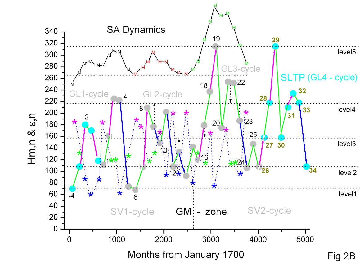
Figure 2B.  Dynamical / evolutionary layer → how the system moves through these states (S-cycle sequencing, transitions, asymmetry, memory). The time axis (x) spans 0–5000 months from January 1700, while the y-axis shows cycle amplitudes Hm, the transition parameter ε (stars) , and the 5-points smoothed memory parameter M̄ₙ. The smoothed evolution of the memory parameter M̄ₙ captures this long-term behavior, providing a continuous representation of the underlying energetic state. The correspondence between M̄ₙ and the large-scale modulation of cycle amplitudes suggests that the Gleissberg cycle can be interpreted as a slow trajectory of the system within the constrained manifold The piecewise linear curve Hmₙ represents the amplitudes of S-cycles, with observed values shown as gray circles and inferred values as cyan circles.

Magenta segments connect members of Hs⬆️ pairs (growth sequences), blue segments connect Hl⬇️ pairs (decay sequences), and green segments link adjacent H-pairs and isolated cycles. The Λₙ curve (stars) shows strong variability and forms three distinct layers: magenta (⟨Λ_g⟩ = 1.86 ± 0.15) corresponding to transitions into growth, blue (⟨Λ_d⟩ = 0.76 ± 0.13) corresponding to decay, and green (⟨Λ_s⟩ = 1.19 ± 0.05) representing a marginally stable regime of solar activity.

The upper panel shows the smoothed evolution of M̄ (5-point average), indicating that GL3 significantly exceeds GL1 and GL2, which are comparable.

This figure shows how the system dynamically explores the manifold. The smooth evolution of M̄ is combined with strongly intermittent changes in Λₙ, which drive transitions between regimes. The coexistence of gradual trends and abrupt switches reveals the adaptive nature of the system: solar activity evolves through continuous energy changes modulated by discrete structural adjustments. In particular, transitions between regimes tend to occur in a structured manner, suggesting that the system retains a form of memory not only in its energetic state, but also in its structural organization.

Morphology thus plays a crucial diagnostic role in revealing the hidden structure of solar activity dynamics. The ordered sequence of S-cycles, MA levels, and H-pairs indicates that solar activity evolves as a dissipative dynamical system whose trajectory moves along a folded slow manifold of a finite-dimensional attractor. Within this framework the Gleissberg cycle is not a simple amplitude modulation of the Schwabe cycles but a manifestation of slow structural evolution of the dynamical state of the system. Grand minima arise when the trajectory becomes temporarily trapped near the saddle region of this manifold. Physically, this behaviour reflects the nonlinear interaction of the surface Babcock–Leighton dynamo and the deep dynamo processes operating in the solar convective zone (SCZ). Their interference generates the hierarchical cyclicity of solar activity and produces the long-term organization of the solar cycle system.

Just a little more, just a tiny bit: what all of this might have looked like from DDST's perspective.

Solar activity can be understood as a hierarchy of interconnected descriptions: (1) the underlying magnetohydrodynamic processes generate coupled poloidal and toroidal fields governed by PDEs; (2) their effective behavior reduces to low-dimensional dynamics on an inertial manifold, forming (3) a structured attractor with saddle and fold geometry; (4) the observed sunspot number is a projection of trajectories on this attractor; and (5) the SG3 normalization extracts a discrete morphological language of cycles with fixed internal timescale. These are five projections of the same system. Their strength lies in the fact that each “sees” something different, while their weakness is that, individually, they provide an incomplete picture. The first three are theoretical, whereas the last two consist of specially processed observations of SSN time series.

Our primary objective is to maximize the potential of known observations to gain a better understanding of the cyclical nature of solar activity. The analyzed SSN time series begins in 1610 (see Fig. 1 in Karak B.B., 2023) and consists of three S-cycles preceding the Maunder Minimum (cycles #(-7), (-6), (-5))—or "grand minimum"—which commenced in 1645, and thirty S-cycles following the conclusion of the GM period (~1703), which, starting from cycle #(-4), form three GL-cycles. The last of the observed S-cycles is the current Cycle #25, beyond which lies the forecast zone for future solar activity. 

Morphological analysis of S-cycles (projection 4) transforms the sunspot record from a mere sequence of numbers into a structured system that reflects the underlying physics of the solar convective zone. The first step in this process involved strong smoothing, which removed high-frequency noise from the signal and transformed the SSN time series into a sequence of smooth SK-shaped S-cycles. This applied to the most recent 25 cycles, whereas the first eight cycles had significantly lower temporal resolution.

The second step consisted in describing each SK-shape using an SG3 approximation, which represents a superposition of three bell-shaped curves corresponding to the rise, saturation, and decline phases of an S-cycle. Each description (SG3 parameter fitting) assigns to a given S-cycle a set of approximately a dozen parameters, effectively performing a parameterization of the S-cycle. The results of the parameterization of S-cycles #1–24 are presented in Table 2 under the assumption of fixed component widths (σ₁,₂,₃ = 16.5 months). Thus, S-cycles differ from one another in duration (T₀), amplitude (Hₘ), as well as in the amplitudes of the components and their relative positions within the cycle—i.e., in their shape (Gestalt) and its asymmetry.

The third step consisted in establishing a specific relationship between the 11-year (S-cycle) and the secular (GL-cycle) components, which led to a typology of S-cycles (with respect to the GL-cycle) and, ultimately, to the discovery of the discreteness of solar activity. This discreteness is expressed in the fact that To exhibits three quasi-discrete (±5%) values, while Hm falls into six quasi-discrete (±20%) levels. Moreover, it was found that the entire set of observed S-cycles can be represented by nine morphological attractors (MA-cycles).

This quasi-discreteness of solar activity shifts the focus of analysis away from a continuous, effectively infinite-dimensional description (projection 1) of the solar convective zone (SCZ), toward a low-dimensional geometric framework, where the dynamics are organized around a finite set of attractors (projection 3). Instead of treating the SCZ as a continuum of states, the system can be viewed as a structured landscape in which evolution proceeds through transitions between a limited number of discrete morphological configurations.

The observed quasi-discreteness of solar activity—manifested in three quasi-stable values of To and six quasi-discrete levels of Hm—suggests that the underlying dynamics are not only low-dimensional but also structured by a finite set of dominant modes that organize the evolution of the system. Rather than representing independent variability, these discrete levels appear to arise from a deeper organizing structure that constrains the accessible states of the solar convective zone (SCZ).

This observation naturally leads to the hypothesis that the effective phase space of the system is governed by a global attractor with a product structure, combining a three-fold organization in the temporal dimension and a six-fold organization in the amplitude dimension. We therefore propose the existence of a global attractor of the form T^3xD^6, where T^3 represents a three-dimensional toroidal structure capturing the quasi-periodic organization of temporal scales, and D^6 denotes a six-dimensional discrete set encoding the allowed amplitude states. In this framework, the apparent complexity of solar activity emerges as trajectories confined to, and evolving within, this structured attractor. The toroidal component reflects the underlying cyclicity and phase coherence of the system, while the discrete component reflects the quantized nature of the morphological states. Transitions between S-cycles correspond to motion along the toroidal directions, while changes in cycle type correspond to jumps between discrete levels in D^6, mediated by the slow modulation associated with the GL-cycle. Thus, the quasi-discreteness observed in the data is not incidental, but rather indicative of a deeper geometric organization: a low-dimensional global attractor that governs both the continuous evolution and the discrete state transitions of solar activity. Moreover, the quasi-discrete nature of solar activity points to the existence of an inertial manifold (projection 2) upon which the global SCZ attractor acquires a T^3xD^6 structure, decomposing into a finite number of morphological attractors (MA-cycles). The dynamics of the solar cycle constitute a trajectory organized by this attractor and guided by bifurcational transitions between its stable components.

In observations—or more precisely, within the morphological framework of solar activity (SA.m)—this structure manifests itself through the existence of distinct morphological structures (MS) and transitions both within and between them. The primary MS that determines the current regime of solar activity is the H-pair of S-cycles. It exists in two forms. The first is the growing Hs⬆️ pair, in which a short cycle is followed by a second, higher short cycle; this configuration defines the growth regime of solar activity. The second is the decaying Hl⬇️ pair, in which a long, high-amplitude cycle is followed by a lower, moderately long cycle; this configuration defines the decay regime. A GL-cycle always begins with an Hs⬆️ pair and ends with an Hl⬇️ pair. The behavior of the two internal H-pairs (as well as the presence or absence of an intermediate single S-cycle between them) determines the structure of the upper dynamical saddle (UDS) of the GL-cycle. The decay of the preceding GL-cycle (Hl⬇️ pair) and the growth of the subsequent GL-cycle (Hs⬆️ pair), together with the single S-cycle separating these H-pairs, form the lower relaxation saddle (LRS). A fifth morphological structure is the grand minimum of solar activity.

To describe this observed slow dynamics, a reduced dynamical framework based on ODEs is employed, in which slow and fast variables coexist, along with critical geometric objects such as saddle points (e.g., LRS and UDS), fold lines corresponding to regime transitions (growth ↔ decay), and separating surfaces (separatrices) that delineate trajectories leading either to regular GL-cycles or to grand minima. 

Structure of the minimal 4D ODE system.  We consider a strongly nonlinear four-dimensional system of differential equations, where the variables x, y form a fast dynamo subsystem; the variables m, c constitute a slow evolutionary layer. Thus, the system belongs to the class of slow–fast dynamical systems with internally coupled subsystems.

dx/dt = c · y -  α · x - β · x^3: Toroidal field x — generation of the toroidal field, representing the efficiency of energy transfer from the poloidal component; linear losses (dissipation); nonlinear saturation limiting amplitude growth. This equation represents a nonlinear oscillator with self-saturation, modulated by the coefficient c.

dy/dt = m · x - γ · y: Poloidal field y — generation of the poloidal field (generalized Babcock–Leighton mechanism), dependent on the system state; decay of the poloidal component. The efficiency of the return transformation is controlled by the variable m, representing the state of the slow layer.

dm/dt = ε · ( δ · x^2 - m) - η · m^3:  Slow variable m (MEC) — energy accumulation (depends on squared amplitude); relaxation toward equilibrium; timescale of slow evolution; nonlinear constraint ensuring saturation and multistability. The variable m acts as a memory variable and a descriptor of slow regime reconfiguration.

dc/dt = μ · (m - c) - ν · c^3: Coupling variable c — tendency toward alignment (adaptive coupling); adaptation rate; nonlinear limitation (dissipation/saturation). The variable c governs synchronization of subsystems, phase relations, stability and possible breakdown of the regime.

Interpretation of Coefficients. Fast subsystem: alpha — linear losses of the toroidal field; beta — nonlinear saturation; gamma — losses of the poloidal field.                          Slow subsystem: epsilon — small parameter defining the slow timescale; delta — sensitivity of MEC to cycle energy; eta — strength of nonlinear constraint on m; mu — adaptation rate of coupling; nu — limitation and degradation of coupling. Structural Interpretation. x, y — fast oscillatory dynamo cycle; m, c — slow variables governing the system’s regime. Coupling structure: x \ m through energy x^2; m \ y (generation control); m \ c (mutual regulation); c \ x (feedback into the cycle).

Physical Meaning: m — accumulation and reconfiguration of deep magnetic energy; c — structural coupling and coherence of flows. Their interaction determines: regime transitions, cycle asymmetry, occurrence of prolonged minima. The system forms a closed loop: cycle energy=memory=structure=cycle generation.

Interpretation of MEC (Magneto–Evolutionary Coupling) is a dynamical mechanism of self-consistent evolution in which magnetic energy determines the structure of flows; the flow structure, in turn, determines magnetic energy generation. Formally, this is: a closed dynamical variable describing the state of magnetohydrodynamic organization of the system. MEC performs three key functions: Energy accumulation x^2 \ m, Structural reconfiguration m \ c, Feedback modulation of the cycle c \ x. MEC is a closed feedback mechanism of self-organization, where the system acts upon its own organization through magnetic energy and flow structure. MEC is a slow dynamical variable describing the configuration of magnetohydrodynamic organization, controlling energy conversion efficiency and flow structure.

This 4D slow–fast ODE model exhibits a rich dynamical and geometric structure, in the sense that it simultaneously incorporates:

1. Scale separation (slow–fast)

• two fast modes
• two slow variables, which already renders the phase space intrinsically multilayered

2. The geometry of the slow manifold

• multiple sheets
• folds
• possible loss of stability

It is precisely within this structure that the following emerge:

• H-pairs
• regime transitions
• asymmetry

3. Multistability

• multiple attractors
• multiple stable cycles, giving rise to:
• discrete cycle durations
• discrete amplitudes

4. A bifurcation structure

• saddle-node bifurcations
• Hopf bifurcations
• transitions between branches, leading to:
• regime switching
• grand minima

5. Intrinsic memory via the variable m

• the system is non-Markovian
• its evolution depends on history

6. Nonlinear feedback closing the self-organization loop (MEC). Thus, the proposed 4D dynamical system possesses a rich geometric and dynamical structure, including slow–fast decomposition, multistability, bifurcations, and nonlinear feedback loops. This structure enables the emergence of multiple coexisting regimes, discrete cycle characteristics, and transitions between them.

Moreover, there are strong morphological grounds to assume that the system operates in a regime of significant effective viscosity. This leads, despite the large number of mathematically admissible solutions, to a substantial contraction of the phase space in terms of realizable trajectories. This situation opens a unique possibility for constructing a practically unambiguous preferred long-term prediction (PLTP) for the entire Gleissberg cycle. Such a trajectory becomes an extremely productive reference framework for further analysis of solar activity. In this context, it is not so much the agreement with the PLTP that is most informative, but rather the deviations from it.

Dynamical analysis of SSN solar activity evolution and formulation of a PLTP for the next Gleissberg cycle. A minimal dynamical representation of solar activity consistent with the observed morphological structure can be formulated as a system that naturally generates folds, saddle structures, canard trajectories, and separatrices, thereby reproducing the full hierarchy of S- and GL-cycle morphology, including grand minima. We begin the interpretation of observations and the construction of the PLTP with the LRS (Lower Regular Saddle).

Passage through the saddle point. Its onset corresponds to the declining phase of the preceding GL-cycle, observed as an Hl-pair. Four such cases have been identified. The first case is (presumably) an Hl-pair after ~1610, followed by the entry of solar activity into the Maunder Grand Minimum. The second case is a sharply declining Hl-pair (cycles #4–5), followed by the formation of MA1.1 (cycle #6). The third case is a weakened Hl-pair (cycles #13–14), followed by the emergence of MA1.2 (cycle #15). The fourth case is a typical Hl-pair (cycles #23–24), again followed by MA1.2 (cycle #25). Thus, passage through the saddle leads to the formation of one of three regimes: MA1.2, MA1.1, or MA1.0. The morphological minimum of the LRS corresponds to the projection of the saddle point, in whose vicinity the trajectory may become “trapped” for an extended period (~60 years), due to the combination of low E and high δ, resulting in an unstable state of solar activity (case 1). In case 2, the trajectory does not become trapped, although it remains near the saddle for a relatively long time. In cases 3 and 4, the trajectory passes sufficiently far from the saddle, leading to the formation of a short and moderately strong MA1.2 cycle. Because the system possesses memory, the configuration at the saddle influences the morphology of the subsequent Hs-pair. In this framework, the saddle is not merely a transient feature of the phase space—it acts as a dynamical gatekeeper of solar activity. It is precisely in the vicinity of the saddle that the system loses stability, amplifies sensitivity to slow variables (E, δ), and selects among alternative evolutionary pathways. The saddle thus performs a dual role: as a separator, it partitions the phase space into distinct morphological basins (MA-regimes); as a selector, it determines which attractor the trajectory will approach after the transition. Grand minima, weakened cycles, or rapid recoveries are not independent phenomena, but different outcomes of how the trajectory negotiates the saddle region—whether it lingers near it, grazes it, or bypasses it at a distance. In this sense, the saddle is the organizing center of regime transitions: it converts slow parametric modulation (GL/MEC dynamics) into discrete morphological outcomes. The apparent intermittency and quasi-discreteness of solar activity thus emerge not from randomness, but from deterministic navigation through a structured phase space whose critical nodes are saddle points. 

Growth phase of the GL-cycle. It may consist of one or two short Hs-pairs. Three distinct growth scenarios are observed. The first occurs after MA1.1 (# −4), immediately following the system’s exit from a grand minimum. Of the three main S-cycle parameters (To, Hm, and asymmetry A), in this case only Hm can be assessed with some confidence, while To can only be inferred. The first Hs-pair in the GL1-cycle takes the form [MA2.1–2.2] (# −3 to # −2). A second Hs-pair [MA2.2–2.1] (# −1 to 0) can also be identified, although it cannot be considered growing (see Fig. 2B). Thus, the growth phase in the GL1-cycle appears to begin, but already in the second Hs-pair a decline sets in (the cycles being short). Cycles #0 and #1 correspond to MA2.1 and MA4*, respectively, with #1 reaching Hm~108. 

The second growth phase also begins after MA1.1 (#6). The first member of the growing Hs-pair is of type MA2.1 (#7), but strongly asymmetric (slow rise, rapid decay). The second member of the pair is MA2.3 (#8), indicating a very rapid growth confined to a single Hs-pair. 

The third growth phase begins after MA1.2 (#15). The first member of the Hs-pair is, as expected, MA2.1 (#16) and relatively symmetric (fast rise, moderately slow decay). The growth rate is slow (progressing from one level to another). The second member of the first Hs-pair (#17) is MA2.2. The process continues over two Hs-pairs, with the second Hs-pair taking the form [MA2.3–2.4]. Three different modes of exiting a low-energy saddle state are described here: weak, intermittent growth (Case 1); sharp, impulsive growth (Case 2); and gradual, multi-step growth (Case 3).

Case 1 — growth begins, but then subsides. Geometry: the trajectory exits the LRS region but remains very close to the separatrix, moving along the unstable direction of the saddle. Dynamics: E is still too small; the system has not yet "detached" from the saddle, giving rise to canard-like behavior: initial growth followed by a breakdown. The observed drop from a moderately high-amplitude state (~158) to a low level (~108), followed by renewed growth, indicates a secondary fold structure on the upper branch. Rather than returning to the saddle, the trajectory undergoes a partial loss of stability and is captured by a lower-amplitude attractor within the upper manifold, from which growth resumes.

Case 2 — short but rapid growth. Geometry: the trajectory passes close to a fold, rapidly jumping between the branches of the slow manifold. Dynamics: E is already higher, but δ remains large → asymmetry; consequently, a slow rise (sticking) occurs, followed by a rapid upward escape. This is a classic canard explosion. Therefore, the first cycle (MA2.1) is asymmetric, while the second (MA2.3) involves an abrupt jump: the system has sharply "leaped" to a higher regime.

Case 3 — smooth, stepwise amplification. Geometry: the trajectory passes far from the saddle and moves along the stable branch of the slow manifold. Dynamics: E increases steadily, δ decreases or stabilizes, and the system transitions sequentially between levels without losing stability; therefore, growth proceeds via two Hs-pairs, and the system is already "within the growth attractor." So, the diversity of GL-cycle growth scenarios reflects different geometric pathways of the trajectory relative to the saddle–fold structure of the slow manifold. Weak, impulsive, and structured growth correspond, respectively, to trajectories that (i) linger near the saddle separatrix, (ii) undergo canard-mediated jumps near folds, or (iii) evolve along stable branches of the slow manifold. Hs-pairs are not merely an observation, but discrete markers of the system's geometric motion. The diversity of GL-cycle growth scenarios is not phenomenological but geometric: it reflects how trajectories, shaped by prior saddle passage, are injected onto different regions of the folded slow manifold. 

Change of growth regime. The morphology indicates two growth regimes of the GL cycle:

(1) rapid and short (less stable GL2), and

(2) gradual and long (more stable GL3).

The GL1 cycle represents a transition GM → GL, while in the first half of the 17th century there was a transition GL → GM.

In both cases, the encounter of the trajectory with a fold interrupts the growth regime, after which a decline is observed. However, the nature of this decline differs.

In the first case, an Hl-pair of the form [MA3.1–4] appears (a transition one level down, from 218 to 158).

In the second case, there is a sharp drop MA2.4 → 4 (a transition two levels down, from 315 to 158).

At the same time, the type of the terminal S-cycle is the same in both cases — it is MA4. During the growth phase (GL2 or GL3), the system accumulates magnetic energy while approaching a fold. At the fold, the configuration reaches its stability limit: further growth becomes dynamically impossible. This triggers a rapid transition in which the accumulated toroidal energy is released, and the system is forced off the growth branch. The trajectory undergoes a downward jump (of one or two levels, depending on the pre-fold energy) and loses its previous structural coherence. As a result, the dynamics collapse into MA4, a low-energy, reorganized state characterized by reduced magnetic complexity and restored stability. In essence: growth terminates at the fold, the system discharges, and the dynamics reset to MA4. After reaching the MA4 level, the system approaches a bifurcation-like threshold. The existing attractor becomes unstable, and the system undergoes a fast jump to a new branch of the phase space. This transition is characterized by a rapid change in state variables, occurring on a timescale much shorter than the preceding slow evolution. As a result, the system does not return to its previous baseline but lands in a new metastable regime with a higher effective energy level. Subsequent S-cycles are then initiated from this elevated state, leading to a systematic upward shift in the cycle baseline. So, the passage through MA4 induces a fast jump: a rapid transition between attractors that reinitializes the system on a higher metastable branch, leading to an elevated baseline for the subsequent S-cycle. 

The second hump and the second jump. As a result of the first fast jump, after the system transitions to the intermediate level MA4, a high first member of a new H-pair is formed. It can be either short or long, depending on the history (memory) of the development of the first hump of the current GL cycle. More precisely, it depends on what the second H-pair of that hump was like.

If it was of type Hs, then the third pair will also be of type Hs; if it was of type Hl, then the third pair will be of type Hl. Accordingly, the tendencies of growth or decline are preserved.

Since the fourth H-pair is always of type Hl, in the case of a prevailing declining trend in the GL cycle, a second fast jump will be required, as happened in the GL2-cycle.

On the fundamental asymmetry of solar cycles. At present, we can more or less confidently reason about two solar cycles: the 11-year cycle (S-cycle) and the centennial cycle (GL-cycle). Each of them is characterized by three main parameters: duration, amplitude and asymmetry with our focus on the structural aspect. The S-cycle has three quasi-discrete values of duration To, and this is quite rigid. Its amplitude is also discrete, but more “softly.” As for asymmetry, it is binary: either fast rise and slow decline, or the opposite — but full symmetry is absent.

The GL-cycle, however, is deeply structured and fundamentally asymmetric. Its basic element is H-pairs of two types. These contrast with single S-cycles, which appear only at extrema: between GL cycles and their humps. The fact that a GL-cycle consists of four H-pairs determines its morphological structure, which is clearly asymmetric. The first H-pair is always of type Hs, while the second may be either type. Given that the fourth H-pair is always of type Hl, we obtain — depending on the type of the second H-pair — an asymmetric structure of either: 3Hs + Hl or Hs + 3Hl. Symmetry is thus forbidden. This feature of S-cycle generation in the self-organized solar convective zone (SCZ) imposes strong constraints on long-term prediction of SSN (solar activity), see Fig.2B.

In turn, our 4D ODE system must be in principle extended to, say, a N-dimensional continuous dynamical system coupled to a discrete switching variable, forming a hybrid phase-coherence model with memory and threshold-driven transitions. This is due to the fact that SCZ is a system with memory, in which a cycle is not an oscillation, but rather a sequence of synchronization modes—transitions between which are rare, yet structurally predetermined events. However, further theorizing falls beyond the scope of this work, which is, in essence, definitely morphological.

                                                                                  Quantized Dynamo Automation (QDA-model) of Solar Activity, version v.1.

The research into the morphology of the SSN time series (1610–present)—a project I have pursued since 2000, with intermediate results published since 2008—initially led to a description of S-cycles using the SG3 approximation. Subsequently, it enabled the parameterization of cycles #1 through #24, ultimately leading to the realization that solar activity possesses a discrete structure, manifested in the alternation of two types of pairs (Hs and Hl pairs) and rarer, solitary S-cycles. Subsequently, beginning in 2024, attempts were made to explain and model this structure using the theory of dissipative dynamical systems (DDS) and finite automata.

As a first approximation (Version 1), the global attractor determining the topology of the dissipative dynamical system underlying the self-organization of solar activity was chosen to be a nine-dimensional object of the form T³ × D⁶—that is, the topological product of a three-dimensional torus and a six-dimensional disk. It corresponds to three discrete durations of S-cycles (120, 138, and 150 months), which reflect the principal periods of the morphological structure of solar activity—namely, the 11-year period of the S-cycle, the ~22-year duration of an H-pair of S-cycles, and the ~44-year period encompassing the transition from a short Hs-pair to a long Hl-pair. The amplitudes (heights) of S-cycles assume six discrete values ​​(levels): zero (corresponding to a grand minimum), ~71 (the first, critically low level), ~108 (the second, low level), ~158 (the third, medium level), ~218 (the fourth, high level), and ~300 (the fifth, very high level). A topology of the form T³ × D⁶ corresponds to a type of organization known as quasi-periodic self-organization (or a multi-frequency quasi-periodic regime). It is a multiply connected attractor with a high embedding dimension. From a mathematical perspective, this implies that the solar activity system is deterministic, yet extremely complex. It is not chaotic in the strict sense (like the Lorenz attractor), but it possesses a "memory" of 18 basic states (3 periods × 6 amplitudes) between which it drifts.

The nature of the transitions between S-cycles in our model is determined by a finite-state machine. The finite-state automaton provides a minimal, dynamically consistent representation of solar cycle evolution as a projection of continuous SCZ dynamics onto a constrained discrete state space. By combining this with morphologically observable constraints (symmetry, smoothness, pairing), we arrive at a total of just two fully viable configurations for the GL cycle: D2—prolonged growth followed by a rapid decline (e.g., the GL3 cycle), and D1—rapid growth followed by a prolonged decline (e.g., the GL2 cycle). Both are asymmetrical (symmetrical configurations are prohibited). A finite-state machine represents the logic by which the Sun selects the mode—specifically, the amplitude and period—in which it will operate over the coming centuries. This explains why the Sun does not descend into chaos: it is rigidly confined within the topology T^3 xD^6, wherein only strictly defined, "quantized" states are possible.

Another critical point lies in identifying the saddle points within the sequence of S-cycles. These points prove to be the solitary S-cycles situated at the minimum between GL-cycles (MA1.x # (-4), 6, 15, 25), as well as the solitary S-cycles forming the minimum between the peaks of a GL-cycle (MA4 # 1, (10), 20). There are simply no other solitary S-cycles. MA4 cycles interrupt the decline of the first peak of a GL-cycle and restore the growth of the subsequent S-cycle (which may be either short (# 2, 21) or long (# 11)).

MA1.x cycles generally play a "strategic" role. If it is an MA1.2 cycle (#15, 25), the subsequent GL cycle will have a D2 configuration. If it is an MA1.1 cycle (#6), the subsequent GL cycle will have a D1 configuration. In the case of MA1.0, a grand minimum ensues…These variants correspond to different trajectories traversing the saddle point. The selection of the saddle point—situated between Gleissberg cycles (the minima of the secular cycle)—as the trigger moment for the automaton constitutes a classic example of critical slowing down in dynamical systems. At this point (MA1.x), the system is in a state of minimal stability. It is precisely here that the slightest changes in accumulated magnetic flux appear to determine whether the system embarks on a new Gleissberg cycle or "collapses" into a Grand Minimum. This model explains why the Sun possesses a "memory": the outcome at point MA1 depends on what transpired throughout the entire preceding Hl-pair.

The model described here—the "Quantized Dynamo Automaton"—represents an attempt to characterize the results of my morphological analysis of solar activity (specifically, the SSN time series) through the lenses of DDS theory and finite automata. The construction of strongly smoothed SSN(t) curves constitutes a one-dimensional reduction of the infinite-dimensional MHD dynamics of the solar convection zone (SCZ), raising the fundamental question of the degree to which this reduction remains conformal to the original system. It seems that the most direct and compelling way to address this question is through a structural long-term prediction (SLTP) of solar activity, as enabled by the QDA model.  As a matter of fact, Solar activity is the result of a "clash" between three global processes: meridional circulation (manifested in the duration of the S-cycle, T₀: 3 values), the generation of TMF (manifested in the height/amplitude of the S-cycle, Hₘ: 6 levels), and the regeneration of PMF (manifested in the magnitude of PMF**: 6 characteristic values)—the nonlinear interaction (involving feedback loops of both signs) of which gives rise to its integral structure, QDA (manifested in the order parameter ε and its three situational—or regime—values).

                                                                                              A Structural Long-Term Prediction (SLTP) of Solar Activity

A distinctive strength of the SLTP approach is that it addresses a fundamentally different question: what should the predicted Schwabe (S) cycle look like? This level of structural predictability is, to the best of my knowledge, not provided by existing methods, including the Precursor Method (PM), the Magnetic Terminator (MT) method, or machine learning (ML) models.

                          Table 3. Results of the Structural Long-Term Prediction (SLTP) for Solar Cycles # 25 -34, based on the QDA-model.

S-cycle # to      QDA       year            To     QDA    Hm     QDA-PMF**/PMF**       QDA             ε         regime        type            site        Status as of 

23        2969        -         1996.4         150   218     187           55              57             1.02         0.97         Λ₁/Λ₂      MA3.1         4Hl.1       May 2026

24        3120     3119   2008.92        138   108     106           67            38.2            1.23        1.98          Λ₂/Λ₃       MA3.2        4Hl.2       May 2026          

25        3252     3257     2020.4         120   158     148           67                -               0.84            -                Λ₁         MA1.2       MA1. 2     May 2026    

26           -          3377    2030.42        120   108        -              67               -               1.23            -                Λ₂          MA2.1        1Hs.1       May 2026

27          -           3497    2040.42        120   158        -              84              -                1.35           -                  Λ₂         MA2.2         1Hs.2      May 2026

28          -           3617    2050.42        120    218       -             106               -               1.54           -                 Λ₃          MA2.3         2Hs.1      May 2026          

29          -           3737    2060.42         120    315       -            126                -              0.66            -                 Λ₁         MA2.4          2Hs.2      May 2026 

30          -           3857     2070.42        138    158        -            67                  -             1.69            -                 Λ₃           MA4             MA4       May 2026

31          -           3995     2081.92        120    218        -            106                -             1.07          -                 Λ₁/Λ₂      MA2.3          3Hs.1      May 2026

32          -           4115     2091.92        120    218         -           106                  -           1.07          -                 Λ₁/Λ₂       MA2.3          3Hs.2      May 2026

33          -           4235     2101.92        150    218         -             55                  -            1.02          -                 Λ₁/Λ₂       MA3.1          4Hl.1       May 2026

34          -           4385      2114.42       138    108          -            39                   -               ?            -                    ?              MA3.2         4Hl.2        May 2026

35          -           4523      2125.92          ?          ?            -            ?                    -                  ?            -                 ?                MA1.x         MA1. x     May 2026                                                            

The first three columns of Table 3 present the observed and predicted start (to) of the S-cycle—first in months relative to January 1749, and then in calendar years. The column labeled To indicates the cycle duration in months, as derived from the QDA. The next two columns display the expected and observed cycle amplitude. The next two columns list the expected and calculated maximums of the Sun's polar magnetic field (PMF**, μT). The subsequent two columns provide the model-derived and calculated values ​​of ε. These are followed by the type of morphological attractor (one of nine) and the position of the cycle within the structure of the current GL-cycle (e.g., 4Hl.1 indicates that S-cycle #23 is the first member (1) of a declining H-pair (Hl.), which is the fourth (4) such pair in the GL3-cycle).                                                                                                                                                                                                        

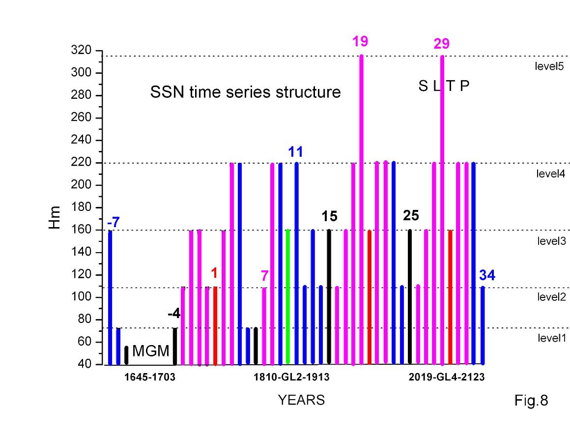
Figure 8. Structural synthesis layer. The x-axis plots time—approximately from 1610 to 2123—while the y-axis plots the amplitudes of the Hm cycles. Each of the 42 S-cycles under consideration (numbered from −7 to 34) is represented by a vertical bar, the structural classification of which is indicated by color. Blue: members of Hl⬇️ pairs (e.g., # (-7) - (-6), #4-5, etc.). Magenta: members of Hs⬆️ pairs (e.g., # (-3) -(-2); # (-1) - 0—tentative; #2-3, etc.). Cycle # (-5) is shown in black and has a height below the critically low threshold (~71, Level 1); it is considered the final cycle prior to entering the MGM period and is therefore classified as type MA1.0 (Level 0, corresponding to activity during the GM period). Cycle # (-4) is considered the first cycle following the exit from the MGM period (like its counterpart, #6, it is also colored black, but has a height of ~71, corresponding to the MA1.1 type). Single cycles of the MA1.2 type (#15 and #25) are also represented by black bars. Their height, Hm, is ~158 (Level 3). The solitary saddle-shaped MA4 cycles (#1, #20, and #30) are shown in red, while the single paired cycle of this group (#10) is shown in green. Thus, the bars display all six height levels of the S-cycles, as well as all four of their types (single cycles in the lower and upper saddles, and short and long paired cycles). 

Based on the morphological analysis presented here, I propose that the solar cycle is not merely an 11-year limit cycle in the Poincaré–Hopf sense, whose parameters are subject to stochastic forcing, but rather a well-defined, more complex phase structure shaped by MHD processes operating throughout the entire solar convection zone (SCZ). Owing to the one-dimensional projection of this MHD system, represented by the smoothed SSN time series, it becomes possible, at least to first order, not only to interpret the observed features of solar activity, but also to construct a structural long-term prediction (SLTP) for the next nine solar cycles (Cycles 26–34). This SLTP serves as a stringent test of the validity of the proposed framework.

While solar cycles #1–24 are now reasonably well established, the structural approach allows us to infer the expected morphology not only of these S-cycles, but, more broadly, of all 42 cycles spanning the period from approximately 1610 to 2123. Let's analyze this structurally: Cycle # (-4) is definitely of type MA1.1—critically low and long. In the quasi-stationary regime of the SA, this would imply that the subsequent GL cycle would be of type D1 (rapid growth followed by a prolonged decline). And cycle # (-3) appeared—specifically type MA2.1—to align with this scenario (its analogue would be cycle #7). Consequently, the subsequent cycle, # (-2), ought to have been short as well, yet high (Hm ~ 218). However, it ended up at the lower boundary (218 – 43.6 = 174.4) of Level 4 ((# -2) ~180), after which something went wrong. The height of cycle (-1) turned out to be even lower: (176 / 1.925) / 75 = 1.219; ((176 / 218) × 98 = 79.119); (125 / 1.925) / 79 = 0.822—an indication not of growth, but rather of a decline phase.

The Y-data do not allow for a sufficiently precise determination of T₀; however, assuming that cycles #(-3)&(-2)—as well as (-1)&0—were short (i.e., the MC had already accelerated and maintained this pace), it must be acknowledged that a configuration switch from D1 to D2 occurred within the 2Hs-pair ((-1)-0) of the GL1 cycle. Consequently, cycle #1—of the MA4 type—formed at the second level (108) (see Fig. 1), after which the SA entered a quasi-stationary regime. Admittedly, the 3Hs pair (2–3) of GL1 proved to be the shortest on record, while the 4Hl pair (4–5) was the longest; however, on average, the situation remained within normal parameters: ((161/1.925)/(65/(158/111)) = 1.832 (indicating strong growth during the transition from #1 to #2). Indirect support for this view comes from the fact that the total duration of the four cycles (–3, –2, –1, 0) is approximately 42 years, as well as from the hypothesis regarding the restoration—following a grand minimum—of synchronization between the deep (GSCB) and surface (BL) levels of the meridional circulation. As for cycles # (-7) through (-5), a structural rationale can be provided for them as well. Cycles # (-7) and (-6) constitute a 4Hl pair of the GL (-1) cycle preceding the MGM, while cycle (-5) is an S-cycle of the MA1.0 type, which was followed by the MGM—an event that can be provisionally designated as the GL0 cycle. This explains the "non-standard" appearance of the GL1 cycle, whereas the characteristics of the GL2, GL3, and GL4 cycles are discussed within the text itself.

                                                                                                     AI Challenge: Deciphering the Solar Engine’s Structural Code

The Quantized Dynamo Automation (QDA) model shifts the paradigm from continuous equations to a structural, state-based logic. To fully validate this framework, I am inviting the AI and Data Science community to address three crucial benchmarks that could confirm the existence of a universal "software" governing stellar activity.

Benchmark 1: Blind Discovery of Phase Attractors

• The Objective: Using unsupervised machine learning on long-term historical and cosmogenic records (e.g., ^ {10} Be\), ^ {14}C\) isotope data), can an algorithm independently identify stable "energy plateaus"?
• The Hypothesis: QDA postulates that the Sun operates on discrete levels (3 for cycle duration \(T_{o}\), and 6 for amplitude \(H_{m}\)).
• The Challenge: Can the AI confirm the existence and exact number of these discrete states without prior prompts?

Benchmark 2: Universal Verification of H-pairs

• The Objective: Apply pattern-recognition algorithms to search for H-pairs (the structural "genetic code" of solar cycles) across two distinct data frontiers:
1. Exoplanetary Data: In stellar activity records of solar-type stars (e.g., Kepler/Gaia missions).
2. Deep Time: Within ultra-long isotopic series, spanning thousands of years.
• The Challenge: Is the H-pair structure a universal constant of the stellar dynamo, and does it remain robust during transitions into Grand Minima?

Benchmark 3: Dynamo Simulations themselves -

Realistic 3D MHD simulations have already demonstrated the spontaneous emergence of coherent magnetic structures, cyclic behavior, and nonlinear regime switching in turbulent solar convection. However, the possibility that such self-organization may also constrain the long-term morphology of solar activity — including preferred cycle-pair organization and restricted secular configurations — remains largely unexplored. 

A Note to Potential Contributors:

I would like to express my sincere gratitude to any researchers, data scientists, or enthusiasts who feel inspired to test these hypotheses. Your insights are invaluable in determining whether these patterns represent a fundamental physical law or a unique structural interpretation. 

Please share your findings: If your models yield results—whether they confirm, refute, or refine these QDA postulates—I would be honored to hear from you. Please reach out to share your data, methodologies, and conclusions. Together, we can decode the rhythm of our Star.

Nick N. Kontor, May 2026.

                                                                                                                          Concluding remarks

1. The 11-year solar cycle (S-cycle), commonly described within the framework of αΩ-dynamo models, is generated within the solar convection zone (SCZ) and thus depends on its current state.
2. The SCZ represents a complex, dissipative, nonlinear dynamical system (DDS), thereby providing the physical prerequisites for the emergence of self-organization.
3. However, complexity, dissipation, and nonlinear dynamics constitute necessary but not sufficient conditions for self-organization. Self-organization emerges only when the system develops persistent coherent structures, constrained transitions, and long-range correlations that reduce the otherwise vast space of possible dynamical states. Chaos by itself expands the space of possibilities, whereas self-organization constrains it from within.
4. The morphology of the smoothed SSN time series examined here in detail provides strong evidence that the SCZ operates as a partially self-organized MHD system, while the observed variability of solar activity reflects the evolution of its internal structure.
5. Thus, self-organization necessarily implies the emergence of structure, understood here as an internal organization of the dynamics that constrains the admissible evolutionary regimes of the SCZ. In the present framework, this structure manifests itself through the existence of H-pairs, discrete Λ-transitions, and the limited set of observed GL-cycle morphologies.                                                                                                                                                                                                                                    I. Basic morphological steps and their results.
6. The SSN time series was subjected to a double - smoothing procedure via high-frequency filtering. As a result, U-data (smoothed data approximating the M-data) and K-data (heavily smoothed yet retaining the asymmetry of the solar cycle) were obtained (see Figs 1, 3, 4).
7. Their description using SG-approximation made it possible to reconstruct the observed forms of Solar Cycles #1–24 (hereafter referred to as SU-shapes and SK-shapes, respectively). The parametrization of the SK-shapes is presented in Table 2.                                                                                                                                      II. Analysis of Table 2 together with the morphology of the three observed Gleissberg cycles (GL-cycles; see Figure 2A) revealed the following properties of the SSN time series:
8. The sequence of S-cycles exhibits a hierarchical structure characterized by a well-defined alternation of four morphological cycle types.
9. The fundamental structural unit of this sequence is a pair of S-cycles (an H-pair, see Fig.6), interpreted here as a manifestation of a particular MHD regime of the SCZ. One type of H-pair (Hs⬆️-pair) consists of two short growing S-cycles, whereas the other type (Hl⬇️-pair) consists of two long declining S-cycles. The short growing cycles correspond to Type 2, while the long declining cycles correspond to Type 3.
10. Solitary Type-1 cycles are located between adjacent Hl and Hs pairs, forming saddle-like transition states between neighboring GL-cycles.
11. Solitary Type-4 cycles — moderately long (~138 months) and moderately strong (~158 SSN) — are located between Hs–Hs sequences near the maximum phase of the GL-cycle, where they form the intermediate depression separating its two peaks (see Fig.2B).
12. The morphology of a GL-cycle is determined by the alternation of four H-pairs, with the first pair always corresponding to the Hs configuration and the fourth pair to the Hl configuration.
13. These constraints strongly restrict the admissible morphology of the GL-cycle, resulting in the existence of only two asymmetric configurations: D1=Hs->Hl->Hl->Hl and D2=Hs->Hs->4->Hs->Hl respectively. Thus, the GL-cycle consists of 9 or 10 S-cycles, the first of which is situated at the bottom of the LRS and takes the form of MA1.x (= 2, 1, 0). This is followed by a 1Hs-pair, and subsequently by 2Hs and MA4—if the configuration is D2—or by 2Hl (the second member of which is also MA4)—if the configuration is D1. Following the MA4-cycle (the bottom of the UMS), growth resumes; in the case of D2, this manifests as 3Hs, while in the case of D1, it takes the form of a 3Hl-pair. The conclusion of the GL-cycle (the 4Hl-pair)—much like its inception (the 1Hs-pair)—is structurally stable.                                                  III. Interpretation of the observed structure of solar activity. By the structure of solar activity, we mean a persistent restriction of the space of admissible MHD regimes of the SCZ, manifested through the existence of preferred states, a limited number of transitions between them, and long-range correlations in the sequence of solar cycles. This interpretation follows naturally from the DDS framework.
14. The morphology of solar activity makes it possible to identify nine types of morphological attractors (MA-cycles). Their SK-shapes are empirically known (Table 2), and each MA-cycle is discretely characterized by three integral parameters — To, Hm, and PMF** — together with a transition operator Λ describing the transition to the subsequent cycle.
15. Their discreteness corresponds to three regimes of deep meridional circulation (MC), six levels of accumulated strong toroidal magnetic field (TMF), six estimated levels of the cycle-integrated polar dipole magnetic field (PMF ~ PMF** (proxy)), and three distinct transition regimes between cycles (the three Λ-values) arising during the adaptive evolution of the system (see Figure 2B).
16. The Λ₂ (~1.25) regime should not be interpreted as a static equilibrium state, but rather as an intermediate transitional regime separating two opposite tendencies of the system: structural amplification (Λ₃ ~1.75) and structural relaxation (Λ₁ ~0.75). In this sense, the observed moderate oscillations reflect the continuous rebalancing required to maintain self-organization within the SCZ.
17. In complex systems theory, persistent structure does not emerge despite variability, but through it. Stability is achieved not by static equilibrium, but by continuous adaptive reorganization sustained by nonlinear feedbacks, memory effects, and multiscale interactions. In this sense, solar activity may be viewed as a self-organized MHD structure of the SCZ, whose long-term variability reflects the intrinsic dynamics required to preserve global coherence (see Fig.5).
18. One consequence of SCZ self-organization is the possibility of structural long-term prediction (SLTP). The principal methodological significance of SLTP lies in the fact that, within the framework of the proposed concept, it becomes possible to infer the approximate structural form of future solar cycles long before conventional forecasting methods can be meaningfully applied to them (see Figs 2B & 8). 
19. Morphological regularities constitute empirical findings. Their interpretation in terms of self-organized constrained dynamics is conceptual, whereas the proposed role of MC, helicity, and αΩ-coupling represents a physical hypothesis intended to explain the origin of the observed structure.

20. Our morphology reveals a distinct structure of global solar activity; however, the extent to which this is corroborated by theory remains an open question.            IV. What Changes in Our View of Solar Activity 

21. Our morphology reveals a relatively simple pattern of solar-cycle variability, whereas a full MHD description contains an effectively enormous number of degrees of freedom (see Paul Charbonneau, Dynamo Models of the Solar Cycle, 2005, 2010, 2020). This gives hope that solar activity may eventually be understood within the framework of complex systems theory, although such an approach is far from simple.                                                                                                                                     

22. We suggest that a preliminary morphological approximation of an effective global attractor of the solar convection zone (SCZ) may be represented in the form: T^3xD^6 where T^3 corresponds to recurrence, cyclicity, and transport rhythm, while D^6 corresponds to structural plasticity, branching, and coherence reorganization.                                                                                                                                                                                                                                                                   

23. We may then describe the dynamics of the solar convection zone as a two-component system: π/scz~MC(t)±i•MEC(t) where: MC (Meridional Circulation) controls the kinematic and transport aspect of the system. It determines flow speed, cycle timing, magnetic-flux advection, and the overall temporal pacing of the solar cycle. In short, MC governs how fast the system evolves. MEC (Multi-scale Emergent Coherence) controls the structural and organizational aspect of the system. It determines the coherence of large-scale coupling, the depth of system memory, phase synchronization across scales, the morphology of cycle structure, and the stability of dynamical regimes. In short, MEC governs how the system is organized while it evolves. Thus, the solar cycle is not determined by a single scalar amplitude, but by the interaction of two quasi-orthogonal components: MC → dynamics (speed / transport) and MEC → structure (coherence / organization). Different cycle types (for example, high and low phases within paired cycles) may therefore be interpreted not merely as amplitude variations, but as transitions between different MC–MEC configurations within the system’s state space. Two cycles with similar amplitudes may belong to fundamentally different regimes if their internal coherence structure (MEC) differs. This leads to a new interpretation of solar activity as a trajectory within a joint transport–coherence phase space, rather than a simple periodic oscillation.                                                                                                                                                                                                                                           

24. Within this framework, MA4 and saddle states may be interpreted as regions where the effective geometry of D^6 becomes weakly constrained, while grand minima may correspond to periods of structural desynchronization (MEC~0). In such states, cycles acquire an MA1.0-like morphology and enter the Λ₂-regime, which appears incapable of sustaining either a stable declining phase or a stable growth phase of solar activity.                                                                                                 

25. The deeper one looks, the stronger the impression becomes that solar activity is not a single cycle, but rather a multilayered self-organizing system with memory, branching behavior, and a hidden geometry of states (see Fig.7).                                                                                                                                                                             

26. At the same time, this system appears to be only partially self-organized: it is neither fully chaotic nor fully ordered. Order emerges locally, temporarily, and in a limited manner, rather than as a perfectly stable global structure.                                                                                                                                                     

27. Morphological analysis of the sunspot number (SSN) time series reveals a number of persistent morphological invariants of solar activity, including forms of organization, transition topology, pattern stability, and an underlying “grammar” of dynamical evolution. These invariants include H-pairing, Λ-transition structure, saddle behavior, allowed and forbidden transitions, asymmetry patterns, and MA classes. Remarkably, the same morphological framework simultaneously admits multiple complementary interpretations of solar activity — spectral, dynamical, geometric, topological, informational, a finite-state machine interpretation and self-organizational. Taken together, these perspectives point toward a solar convection zone (SCZ) that behaves not as a simple oscillator or purely stochastic turbulent medium, but as an adaptive, partially self-organized, multiscale MHD system with constrained morphology, distributed memory, evolving coherence geometry, and topology-dependent transitions between metastable dynamical regimes. 

28. From this perspective, solar activity may not be intrinsically “complex” in an absolute sense. Rather, complexity may reflect the present limitations of our descriptive framework. In this view, complexity is not necessarily a fundamental property of nature itself, but a property of the relationship between a system and the language used to describe it. What we call a “complex system” may simply be a system for which the natural collective variables, symmetries, and organizing principles have not yet been identified — variables capable of compressing enormous, microscopic complexity into a simpler effective description. Solar activity may therefore represent not merely a sequence of isolated cycles, stochastic fluctuations, or the output of a single dynamo mechanism, but the observable projection of a deeper multiscale organization within the SCZ. In this sense, the proposed morphology may serve not only as a classification scheme for solar cycles, but as an attempt to identify the natural descriptive coordinates of the system itself — the effective variables governing its collective organization, memory, coherence structure, and admissible transitions between dynamical regimes.                                                                                                                                                                                                                                                                                                                    ἐπίλογος: In sulcis praeteriti nascitur iter futuri. ChatGPT 

    §1. Periodicities of Solar Activity (a Spectral approach)

     Spectral analyses of various solar-activity time series reveal a broad set of periodic components spanning a wide range of timescales. In the review by N. N. Kontor (1993), the most prominent periodicities included the ~11-year Schwabe cycle, the ~22-year Hale magnetic cycle, the ~88-year Gleissberg cycle, and the ~200-year Suess–de Vries cycle. Numerous studies have subsequently reported additional periodic and quasi-periodic components on both shorter and longer timescales.

     The morphological framework considered here suggests the existence of a hierarchical organization of characteristic timescales. In particular, several observed periods appear to be approximately related through a binary scaling relation of the form Tn ~ To•(2^{±n}) [1], where To denotes a characteristic reference timescale (~11 years). Although this relationship should presently be regarded as a phenomenological observation rather than a demonstrated physical law, it points to a possible hierarchical ordering of temporal structures within solar activity.

    From this perspective, solar activity appears not as a process characterized by a single dominant cycle, but as a multiscale system in which different levels of variability may be dynamically interconnected. The origin and physical significance of these apparent scale relations remain open questions.

    §2. Identification of the S-Cycle (A Geometric approach)

    Strong smoothing of the sunspot-number record preserves only morphological structures corresponding to characteristic timescales with n > (or equal)-1 in the adopted hierarchy. Within this representation, an individual S-cycle can be characterized by four principal attributes: 

    1. Cycle length (To~ 120, 138, or 150 months);
    2. Cycle amplitude (Hm ~ 0, 71, 108, 158, 218, or 315);
    3. Shape asymmetry, typically expressed as a relatively rapid rise followed by a slower decay of varying duration;
    4. The overall SK-shape, which may be parameterized using an SG3 approximation.

     To first order, S-cycles may be distinguished or grouped according to any combination of these four characteristics.

     A notable feature of the identified S-cycles is the apparent discreteness of both their lengths and amplitudes. From a geometric perspective, this suggests that the observed cycles occupy a limited set of preferred regions within the space of morphological states rather than forming a continuous distribution. Whether this discreteness reflects an underlying low-dimensional organization of solar activity remains an open question, but it provides a useful phenomenological basis for further analysis.

    §3. Typology of S-Cycles and Long-Term Memory (A Dynamical and Morphological Perspective on SCZ Memory)

     At its core, the typology of S-cycles addresses the question of memory within the solar convective zone (SCZ), denoted here by π. Such memory may be classified as internal or external, flow-related or structural, and short-term or long-term. The intrinsic memory of the  αΩ-dynamo is generally regarded as short-lived and has been extensively discussed in reviews of solar dynamo theory (e.g., Charbonneau, 2020). In contrast, the morphology of the sunspot-number record suggests the existence of a longer memory component within the SCZ.

     The most prominent evidence is the recurrent formation of H-pairs of S-cycles. Two principal types are identified:

    • Hs-pairs, consisting of two relatively short S-cycles associated with a rising activity trend;
    • Hl-pairs, consisting of two long S-cycles whose amplitudes and durations both decrease from the first cycle to the second.

     Between successive H-pairs, one or two isolated S-cycles are frequently observed. Morphologically, these cycles appear to be associated with saddle-like states of the system and therefore may be interpreted as transitional structures linking neighboring H-pairs.

    This organization implies that the evolution of a given S-cycle cannot be understood solely from its immediate predecessor. Instead, the observed sequence suggests a memory extending over at least two or, may be, three Schwabe cycles (~22 years or longer).

    The saddle-like states correspond to the lower regions of large-scale morphological saddle structures. In the LRS configuration a saddle cycle is always present, whereas in the UMS configuration its occurrence depends on the specific Gleissberg-cycle morphology (D1 or D2).

    As a phenomenological representation, the memory of the SCZ may be expressed symbolically as π = MC± i•MEC [2], where MC denotes flow-related memory and MEC denotes structural memory. Within this framework, the observed morphology suggests that under certain conditions structural memory may dominate overflow memory, thereby influencing the large-scale organization of solar-cycle sequences.

    At present, the physical origin of this apparent structural memory remains uncertain and should be regarded as a working hypothesis rather than an established property of the solar dynamo.

    §4. The Nature of the Gleissberg Cycle (A Combinatorial Perspective)

    The memory of the solar convective zone (SCZ) generates connections both within and between H-pairs, while transitions among them appear to be constrained by the geometry and topology of the system’s phase space.

    The morphology of the sunspot-number record indicates that, following a minimum of activity, the recovery phase typically begins with an Hs-pair. This pair is followed by a second H-pair, which may be either Hs or Hl. In the former case, activity continues to rise, whereas in the latter case a local activity hump is formed. Subsequently, growth temporarily slows or ceases, but later resumes. Depending on the preceding evolution, this renewed development takes the form of either another Hs-pair or an Hl-pair associated with declining activity. The final Hl-pair completes the full sequence known here as a Gleissberg (GL) cycle.

    Three complete GL-cycles can be identified in the historical sunspot-number record. Although each cycle is unique in detail, their morphology appears to reduce to only two fundamental configurations, denoted D1 and D2. Both are asymmetric structures composed of four internally coherent H-pairs. The constituent H-pairs are morphologically similar within a given configuration but differ systematically between D1 and D2.

    Within this framework, the Gleissberg cycle is interpreted not simply as a secular modulation of Schwabe-cycle amplitudes but as one of two admissible asymmetric configurations formed by four interacting H-pairs.

     §5. Topology of the Morphological State Space

    Combining the discreteness of S-cycle parameters with their position within the Gleissberg-cycle framework leads to the notion of a strongly constrained phase-space topology of the SCZ. Morphologically, the observed diversity of solar cycles appears to collapse onto a limited set of preferred states represented by nine morphological attractors (MA-cycles).

     This suggests a hybrid branching structure in which the long-term evolution of solar activity follows a restricted set of admissible trajectories. In particular, transitions between consecutive GL-cycles frequently occur through a large relaxation saddle (LRS) configuration of the form (Hl - MA1.x - Hs). The subsequent evolution depends critically on the state x. If x=2, the following GL-cycle is expected to evolve toward a D2 configuration; if x=1, toward D1; whereas x=0 corresponds to the onset of a grand-minimum state. From the perspective of dynamical-systems theory, these alternatives may be interpreted as different passages through a saddle region followed by divergence along distinct unstable trajectories. Such behaviour would require both long-term memory and strongly constrained transitions between cycles and H-pairs.

    Although these assumptions cannot be justified a priori, the observed morphology appears remarkably consistent with such an interpretation. Consequently, the hypothesis ultimately remains testable only through future solar-cycle evolution.

    §6. Transitions Between Cycles and Pairs

    Transitions between cycles and H-pairs constitute the central element of the proposed framework because they directly reflect the internal organization of the system. While every transition necessarily occurs, the morphology suggests that it does so according to specific structural rules.

    Each S-cycle is characterized by four integral parameters: (To, Hm, PMF**, ε), where To is the cycle length, Hm is the cycle amplitude, PMF** is a proxy for the polar poloidal magnetic field generated during the declining phase of the cycle, and ε is a transition coefficient describing the efficiency of transfer from one cycle to the next. Using this representation, transitions may be expressed phenomenologically as H{m+1} ~ 1.925•ε•PMF**m [3]. The parameter ε encapsulates the transition rule linking successive cycles and is not known a priori. Particular importance is attached to the highly sensitive MA1.x state. Provided that x≠0, both MA1.1 and MA1.2 are followed by a short and relatively weak MA2.1-type cycle (identified here with Cycle 26). However, the subsequent evolution differs substantially.

    For MA1.1, the system enters a rapid-growth regime Λ₃ with ε approaching its maximum value of approximately 2. For MA1.2, the system instead remains in a declining regime Λ₁, characterized by ε~0.8. These alternatives may be interpreted dynamically as different realizations of a saddle-point crossing projected morphologically onto the floor of the LRS structure. More importantly, the initial condition appears to influence not only Cycle 26 but the entire first Hs-pair, including Cycle 27. This behaviour constitutes a possible manifestation of long-range structural memory within the SCZ. In the rapid-growth scenario, Cycle 27 is expected to become a high-amplitude cycle. In the alternative scenario, the system transitions from the declining regime Λ₁ into an intermediate regime  Λ₂, which approximately preserves the existing level of activity and allows only modest growth or decline depending on stochastic forcing and H-pair type.

    At present, solar activity appears to be located near the bottom of the LRS structure in the form MA1.2 (Cycle 25). Under this interpretation, Cycle 27 is expected to become moderately strong (MA2.2, level 3), corresponding to a slow-growth phase of the next Gleissberg cycle. Consequently, the forthcoming GL-cycle is predicted to resemble the previous GL3 - cycle that ended with Cycle 24.

    §7. Conclusion

    The morphological interpretation proposed here will undoubtedly appear speculative to readers unfamiliar with the long process of extracting and classifying structures from the historical sunspot-number record. Nevertheless, the inferred organization of the solar convective zone appears sufficiently coherent that it cannot be dismissed without examination.

    The proposed structures are not naturally captured by conventional MHD modelling because they are formulated at a much lower effective dimensionality. Nor can they be readily confirmed or rejected by purely statistical approaches, whose methods generally require larger ensembles than those available in the historical record of solar cycles.

    The qualitative dynamical-systems perspective appears better suited to the problem, although the available observational record remains too short for definitive conclusions. As a result, the physical interpretation of the observed morphology necessarily remains tentative.

    The central hypothesis advanced in this work is that solar activity is neither a purely random process nor a strictly periodic system. Instead, it is a turbulent nonlinear MHD system exhibiting elements of self-organization and long-term structure. In this view, self-organization is present but remains partial, stochastic, and multiscale in nature.

    A testable consequence of this hypothesis is the structural forecast proposed for Solar Cycles 26–34. Future observations will therefore provide a direct means of evaluating the validity of the morphological framework developed here.

    References: 

Galileo Galilei “Letters on Sunspots (Istoria e Dimostrazioni intorno alle Macchie Solari)”, 1613.

Eddy, J.A., “The Maunder Minimum”, Science, 1976

Schwabe, H. “Solar Observations During 1843”, (Astronomische Nachrichten, vol. 20., no. 495, 1843)

Wolf, R., “Mittheilungen über die Sonnenflecken”(1851–1860s)

Choudhuri, A. R., “Nature's third cycle: a story of sunspots”, 2015, Oxford University Press

S. K. Solanki, I. G. Usoskin, B. Kromer, M. Schussler and J. Beer, “Unusual Activity of the Sun during Recent Decades Compared to the Previous 11,000 Years,” Nature, Vol. 431, No. 7012, 2004, pp. 1084-1087

I. Usoskin1⋆, T. Chatzistergos2⋆, S. K. Solanki2, N. Krivova2, G. Kovaltsov3, N. Brehm4, M. Christl4 and L. Wacker4 «Sunspot cycles for the first millennium BC reconstructed from radiocarbon », A&A, 698, A182 (2025)

Krist ́of Petrovay,  “Solar cycle prediction”, arXiv:1907.02107v2 [astro-ph.SR] 4 Mar 2020. 

Dibyendu Nandy, "Progress in solar cycle predictions: sunspot cycles 24 - 25 in perspective", arXiv:2009.01908v1 [astro-ph.SR] 3 Sep 2020.