MORPHOLOGICAL RESULTS
This section presents the results of a comparative analysis of the parameters of S-cycles observed since March 1755 (month #75). The section begins with Fig. 1, which shows the view of S-cycle #1 (M-data), its SK- and SU-shapes, and ends with Fig. 3, showing not only the view but also the Precursor Method's (APM) forecast for S-cycle #24. In between, Table 2 (13x24) and fig.2A are shown, where the numbers (parameters of SK-shapes) obtained using the SG3-model are arranged and discussed.
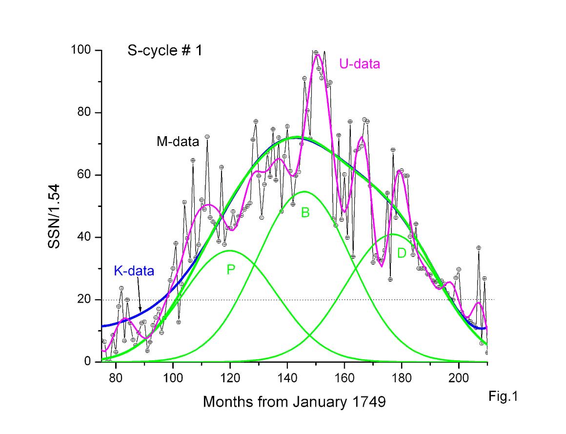
Figure 1 shows an example of the description of the K-data (blue) for the S-cycle # 1 (see table 2) by the SG3-model (green). It can be seen that the model describes well (indistinguishably by eye or with χ2 < 0.1) only the active phase of the S-cycle (when SSN more than ~ 30). One can see three components of the SG3 - model: the first P (t), the second B (t) and the third D (t). It is a low, not very long S-cycle because Hb > Hp and To= 135 months. It is "a high saddle" MA4-cycle. U-data (magenta) allow you to see to what extent they approximate M-data. Four sU-peaks can be seen, the most pronounced of which is sU2-peak. The basic component of the SG-model has the form Gi(t)= Hi • exp {-2•[(t-Xi) ^2]/ (Wi (^2))} (see (2) in part_1).
Table 2 of S-cycles parameters
to +X p - W p - H p = +X b - W b - H b = + X d - W d - H d = T o χ² ≈ 0.1 S- cycle # H m at tm
75 + 47.9 - 33 - 60 = +73.3 - 33 - 80= +103.3 - 33 - 61 = 135 = + (63/31) # 1/MA4 111 = 143
210 + 35.3 - 33 -118 = + 54.5 -33 - 62 = + 78.6 - 33 - 67 = 109 = +(52/30) #2 161 = 252
MA2.2 + 39 - 33 - 116 = +62 - 33 - 88 = + 87 - 33 - 51 = 120 - # 2, 17 158 = 49
318 + 37.1 - 33 - 161 =+ 52 - 33 - 83 = + 84.4 - 33 - 48 = 111 = + (182/38) #3 225 = 359
MA2.3 + 38.3 - 33 - 174 = +59 - 33 - 105 = + 87 - 33 - 56 = 120 = + # 3, 8, 18, 21, 22 218 = 45
429 +39.1 - 33 - 192 = + 64.4 - 33 - 80 = +96 -33 - 77 =132.6 - 33 -30 = 164 = 0.16 (115/0) #4 222 = 471
MA3.1 +41.3 - 33 - 146 = + 67.6 - 33 - 107.5 = + 101.3 - 33 - 53 = 150 = # 4, 9, 11, 23 218 = 50
593 + 42 - 33 - 46.5 = + 72 - 33 - 52.7 = + 92 - 33 - 27.3 = 151 = + (15/15) # 5 74 = 664
744 + 53 - 33 - 33.3 = + 79 - 33 - 55.6 = +114 - 33 - 15 = 149 = + (20/25) # 6 68 = 816
MA1.1 +44.5 - 33- 33.5 = + 72.8 - 33 - 54 = + 95.7 - 33 - 25 = 150 = # 5, 6 70 = 73
893+ 44 - 33 - 53 = + 71 - 33 - 67.5 = + 93 - 28.3 - 68 = 126 = + (30/30) # 7 108 = 975
MA2.1 + 38.9 - 33 - 62.2 = + 61 - 33 - 67.2 = + 88.7 - 33 - 67.6 = 120 = # 7, 16 108 = 57
1019 + 38 - 33 - 169= + 61.4 - 33 - 89 = + 94.3 - 33 - 48 = 116 = + (103/30) # 8 209 = 1062
1135 + 46.9 - 33 - 112 = + 70.8 - 33 - 116 = + 105.4 - 33 - 62 = 149 = + (98/80) # 9 176.5 = 1194
1284 +44.2 - 33 - 117 =+ 68.8 - 33 - 74 = +104.7 - 33 - 59 = 135 = + (75/32) #10 /MA4 149 = 1335
1419 + 40.4 - 33 - 152 = + 62 - 33 - 91.6 = + 93 - 33 - 35.7 = 141 = + (72/12) #11 201.6 = 1465
1560 + 28 - 33- 45 =+ 56 - 33 - 88 = + 83 - 33 - 38 = 135 = + (20/25) #12 108 = 1614
MA3.2 + 34.8 - 33 - 56 = + 60.3 - 33 - 75 = + 85.5 - 33 - 39 = 138 = # 12, 14, 24 108 = 56
1695 + 39.4 - 33 - 113=+ 65.9 - 33 - 59 = + 103.9 - 33 - 29 = 143 = + (130/15) #13 133 = 1738
1838 + 35.5 -33 - 69 = + 63 - 33 - 69 = + 86.5 - 33 - 42 = 138 = + (27/31) #14 92 = 1889
1976 + 39.4 - 33 - 83 =+ 60.8 -33 - 89 = + 89.8 - 33 - 27 = 120 = + (10/20) #15/MA1.2 142 = 2027 (51)
2096 +35.5- 33 - 68.7 = + 57.7 - 33 - 78.5 = + 85.3 - 33 - 38.7 = 122 = + (26/28) #16 120 = 2145
2217 + 42 - 33 - 120 = + 64 - 33 - 99 = + 96 - 33 - 56 = 125 = + (35/22) # 17 179 = 2269
2342 + 42.2 - 33 -178 = + 64 - 33 - 105= + 90.4 - 33 - 66 = 122 = + (109/77) #18 237 = 2390
2464 + 40.2 - 33 - 235 = + 62.6 - 33 - 148 = + 95.8 - 33 - 49 = 126/120 = + (150/60) #19/MA2.4 315 = 2510 (46)
2590+38 -33 - 115 = + 62.8 - 33 - 110 = +93.5 - 33 - 70 = 140 = + (54/89) #20/MA4 175 = 2640
2730 +38.4 -33 -164 =+ 59.4 - 33 - 141 = +87.2 -33 - 73.4 = 123 = + (57/68) # 21 253.5 = 2778
2853 + 35.1 -33 -183 = + 56.8 - 33 - 120.3 = +81.1 - 33 - 52.2 = 116 = +(112/33) # 22 251.6 = 2895
2969 + 36.5 -33 - 91.6= + 61 - 33 - 138 =+87.5 - 33 - 59.4 = 151 = +(57/79) # 23 186.7 = 3024
3120 +38.5 - 33 - 60.9 = + 63 - 33 - 70.7 = + 84 - 33 - 27.7 = 132 = + (15/25) #24 106 = 3176
In table 2, the first column indicates the start of the S-cycle to, the value of which is equal to the number of months that have passed since January 1749. S-cycle duration (its length in months) To, i = to, (i+1) - to, i (see column 11).
Detail # 1. According to their duration, S-cycles fall into two groups - long (To ≥ 132 months) and short (To ≤ 131 months). In drawing this formal boundary, we consider #24 to be long for reasons of assumed by us orderliness of the GL-cycle. This is a very important distinction and was later refined as follows. For short Ss - cycles, To,s = 120±6 months; among long Sl - cycles, we distinguish moderately long (To,l* = 138±4 months) and long (To,l = 150±8 months) cycles.
Between the first and elevens columns, the values of the parameters of the three components of the S-cycle are shown (three for each component, see expression (2) in part_1). The first parameter is the moment of maximum of the component (X p, X b, X d, columns 2, 5, 8 correspondingly).
Detail # 2. The second parameter (Wp ~ Wb ~ Wd ~ 33 months, see columns 3, 6 and 9) determines the width of the P, B and D-components slightly above its half-height (Wi = 2•σt). We can say that this is the main parameter of the SG3 - model, since To ~ W+W+W+W =132 months (11 years). Here the first term is ~ X p, the second and third terms are the “distance” between the P&B and B&D components, and the last term is ~ Wd. The question is: where does W ~ 33 months come from? This is a consequence of my interpretation of the meaning of the second harmonic of the main 11-year FAS peak at a frequency of ~ 0.015 (1/month). I assume that this small peak in FAS indicates the presence of some ~ 66-month periodicity in K-data, which I model with a G (t) function with W = 33 months. I would like to know what is its physical meaning and why does the S-cycle need exactly three such K-peaks in order to take place? (for a possible answer, see the next page). Also, to what extent are they related? (see section III). By the way, all S-cycles (and there are 24 of them) can be described by the SG3 - model with all Wi = 33 months, and only for S-cycle # 4 (the longest one) the description by four “typical” components would also look natural (see Fig. 1 in [1]). Columns 2, 3 and 4 refer to the P - component of the S-cycle. Column 4 gives the height (H p, i) of the P-component. The plot of H p, i where i is the serial number of the S-cycle, is shown in Fig.2A.
Detail # 3. It turns out that the plot of H p, i can be described by the SG2- model, and the resulting two-hump curve, resembling the Gleissberg secular cycle, can be called the GL-cycle, which will play one of two main roles for us (the other is clearly the S - cycle). Figure 2A is important because it highlights the relationship between the 11-year Schwabe cycle and the Gleissberg secular cycle. W. Gleissberg himself (1939) called his cycle 88 years, which suggests the participation of eight S-cycles or four H-cycles (22-year Hale cycles). This remark will be useful to us later.
Columns 5, 6 and 7 refer to the B - component of the S-cycle. Column 7 gives the height of the (H b, i) B - component. Here it must be said that fitting K-data for each S-cycle (due to the large number of free parameters) can be ambiguous. This circumstance required the introduction of some restrictions on the mutual behavior of the parameters, the fulfillment of which increased the reproducibility (stability) of the fit.
Detail # 4. In the process of fitting, a regression of the form H b, i ~ 54 + 0.28•H p, i is found, from which it follows that the height of the S-cycle has a minimum limit Hm, min~54. In addition, it becomes possible to distinguish between low (if Hp < Hb) and high (if Hp > Hb) S-cycles. A boundary between them takes place at Hp = H b ~ 75, what corresponds Hm ~ 140 (see fig.4).
Detail # 5. The P-component determines the phase of the S-cycle growth and largely determines its type (low or high). The B-component (together with the P-component) determines the phase of the S-cycle maximum, and for low S-cycles it is the base one. The D-component (see columns 8, 9 and 10) is a "dark horse" that determines (together with the B-component) the S-cycle decay phase and its length (via Xd). In addition, Hd can play a significant role in the α - effect, but more on that later. To finish with the development phases of the S-cycle, it should be noted that long cycles may have a certain “tail” that does not have a pronounced shape, the length of which is Δt ~ To - (X d +W d). Only #4 has this tail looking like a normal G-peak.
In the process of fitting the shape of the S-cycle, there are "pitfalls" - not all cycles look regular (R, such 6 or 25%). Almost regular S-cycles (R m) require some masking of the beginning and/or end of the active phase of the cycle (5/21%). For cycles with a distorted shape (D), it is typical for some parameters to go beyond one σ (6/25%), and for some, especially distorted ones (D m), masking (7/29%) must also be added. But at the same time, all 24 S-cycles with the parameters indicated in Table 2 are well described by the SG3 - model. What follows from this is still unclear, but the information is briefly presented in columns 12 and 13. The next two columns give the values of Hm at t m, which are determined numerically in the SG3 - model.
Detail # 6. Precursor method (PM/WO) allows to predict S-cycle maximum (Hm+) from PMFm with ±10% accuracy (Hm+ ~ 2•PMFm). Relying on it, we introduce the “reverse” PMF*= Hm+/2, which can be applied to each S-cycle, starting from # 1 (see Fig. 1), and try to describe the growth phase of PMF after t pr by the regression function PMF**(t ) ~ 70•(Σ Mi-data)/((ΔT)^2) μT, where [1< i = t < ΔT= To - t pr] months. Then the observed PMFm= ε • PMF**m, where the second term is my quantitative PMF estimate for the S-cycle decay phase and ε is a coefficient that shows how much the actual α-effect in each case differs from the one predicted by this regression (it can be close to 1 (coinciding is good), about 0.5 (a noticeable overestimation of the α-effect) or 1.5 (and even 2), and this is already a gross underestimation of the α-effect), see Fig. 6 in [1].
Detail #7 is presented in Fig. 2A, where the scatter plot Hp,i (t) with i = 1 - 24 is described by the continuous SG2-model, which introduces both quantitative and structural (component) aspects into the representation of the Gleissberg cycle. If my estimates for S-cycles ## - 3, -2, -1, and 0 are realistic, then after the end of the Maunder Minimum in ~ 1700 (S-cycle # -4), three double-humped secular GL-cycles were observed, as it was still suggested by W. Gleissberg. The humps forming the GL-cycle are closer to each other, while the neighboring humps of different GL-cycles are further apart from each other (see below).
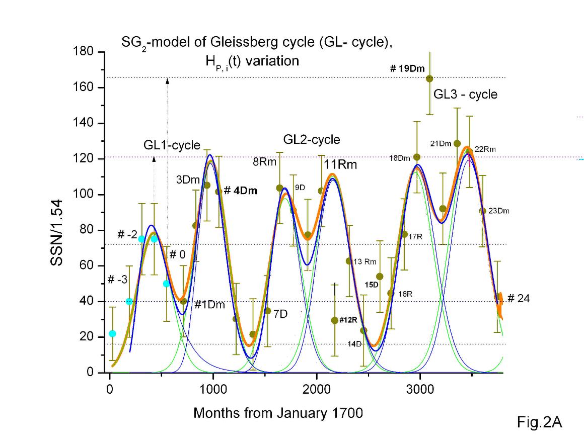
Figure 2A. As already mentioned in "Detail 3", the data in Table 2 allows you to build a scatter plot H p, i (t) for S-cycles # 1 - 24 and even supplement it with S-cycles # - 4 - 0 (see in Fig. 2A cyan points). To give this graph a continuous form, convenient for further consideration, for clarity, I described the points of the graph by G (t)-peaks (see table 1 in part_1), orange and lognormal peaks LN (t), blue. It turned out that the points H p, i seemed to be strung on the curves of these peaks. The peak parameters were fitted with the condition that all points within the error lie on the curve. This condition determined the magnitude of the error ±20 but turned out to be only partly feasible (it did not hold for S-cycles #12, 15, 19). As for the rest, three ~ centennial two-hump cycles were obtained (let's call them GL-cycles); the idea of their similarity with the Gleissberg cycle is coming to mind first. This approach made it possible to obtain a visual description of the current SA episode, which reportedly began in 1645 with the Maunder GM - period after which three GL - cycles appeared one after the other, the train of which continues to the present.
It can be said that a continuous SG2 - model (having form {Xc1 - W1 - H1 = Xc2- W2 - H2} was applied to the discrete graph H p, i (t), the parameters of which for each GL - cycle are given below (Xc & W in years):
GL1: 1735.4 - 27 - 120 = 1782 - 26 - 182
GL2: 1841.8 - 27 - 152.5 = 1879.8 - 28 - 169.4
GL3: 1946 - 29 - 172.5 = 1987.3 - 29 - 186.3
GL4: 2050 - 28 - 167.3 = 2091.4 - 28 - 167.3. This last GL4-cycle (see fig.2B) will be discussed later.
Detail # 8. As a result, instead of a discrete graph Hp, i (X p, i ), a continuous GL-curve (t) is obtained, which is, as it were, a carrier for all possible H p, i within the framework of the SG-model. The presence of the GL-curve takes the consideration of solar activity into a new dimension, as it were. Now we can consider S-cycles and their properties depending on their position on the GL-curve.
The analysis of Table 2 revealed 8 details regarding the values of SK-shape parameters, which are presented as consequences of the data in Table 2. Two of them (Details #7 and 8) discuss the course of Hp,i (t), the description of which by the SG2 - model represents the double-hump view of the three observed Gleissberg cycles (GL1,2,3-cycles). The result is that the S-cycle fits into the structure of the GL-cycle in such a way that the position of each S-cycle on the corresponding GL-cycle becomes known (Fig. 2A). From this point on, each S-cycle is considered with respect to its relationship to the Gleissberg cycle. Consideration of K-data leads to the idea of a relatively complex, albeit “smooth” form of the 11-year S-cycle, behind which are not fully understood processes in the SCS (Solar Convection MHD System in the SCZ) responsible for cyclical changes in SA on a decadal scale. When we turn to the Gleissberg secular cycle, cycles of even greater duration are added, namely, 22-, 44- and 88-year cycles, also generated in the bowels of the SCS.
SGu - model of the S - cycle. If we turn to the consideration of the course of U-data, then its description requires narrower (high-frequency) Gu-functions, which can be called 16-month (~1.3 year) U-peaks (their parameters can be found in Table 1 in part_1 and they can be viewed in Fig. 1, 3, 4, 4A). Then the shape of the S-cycle will no longer be described by only three Gk-components, but by about dozen Gu-peaks (or simply U-peaks) represented by the SG(n)-model. In essence, we obtain the “fine structure” of the S-cycle, which complements the SG3 - model with important details (for example, the appearance of (super) sU-peaks near X p, X b and (to a lesser extent) X d). The solar cycle (11-year S-cycle) not only has an amplitude (Hm (t m)) and duration (To), but also a shape (SK- & SU-shapes) and structure, i.e., a set of interacting elements that together form a whole. In the SG3-model, there are three structural elements, the Gk-components (P, B, D), each with three parameters. In the SGu - model, there are around 12, though they share the same mathematical form.
Figure 3 shows the appearance of S-cycle #24, whose forecast I made in 2006 (Hm=70±17.5, Mold - data, though today this would be ~106 (W.D. Pesnell, 2016, fig. 2). The forecast for Hm was correct, but To was overestimated due to the assumed Xd and Hd. This led to a slowing of the predicted declining phase of the cycle compared to the observed one. This structural mismatch between the forecast and observations highlights the complexity of the process of emergence and development of each S-cycle. This process includes: (1) the ω-effect, in which differential rotation somewhere close to tachocline starts to generate TMF from compressed and strengthened PMF; (2) dynamo waves, which push magnetic tubes (future spots) to high heliolatitudes, forming the P-component; (3) meridional circulation, which ensures Spörer's law by shifting the TMF upwelling zone towards the equator and also transporting PMF to the poles; (4) TMF buoyancy in the CZ, which is subject to turbulent convection and ultimately results in the observation of Hm(t m); (5) helical turbulence, the Brownian motion of spots under the pressure of granules and meridional circulation, all of which together form the α-effect. We know less than we would like about each of these main sub-processes and their interactions, which makes forecasting solar activity challenging.
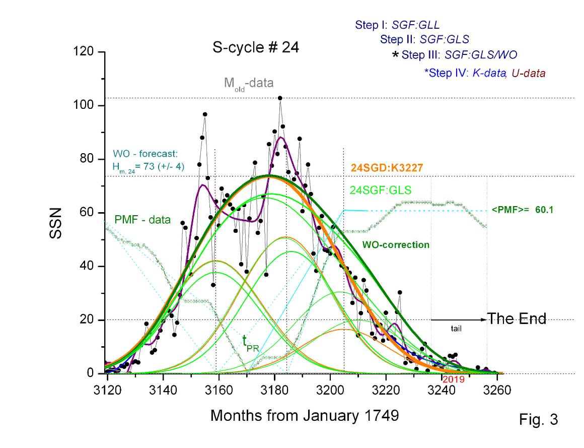
Figure 3 shows the forecasting process and the actual appearance of S-cycle #24. It is MA3.2-cycle.M-data, U-data, K-data (orange), and PMF-data (olive) are displayed. The final 24SGF (dark green) gradually changed "under the pressure" of incoming M-data from green to orange.
Discreteness of the Solar Cycle Morphology
Solar activity originates in the solar convective zone (SCZ), where plasma dynamics obey magnetohydrodynamics (MHD). Its fundamental description is given by a system of partial differential equations (PDEs). This constitutes an infinite-dimensional system in which the variables are physical fields defined at every point in space. Thus, the physical aspect of solar activity, as treated within the framework of the αΩ-dynamo theory, can be formulated as the study of an infinite-dimensional dissipative MHD system of the solar convective zone governed by nonlinear partial differential equations. The solutions of these equations are continuous functions. However, the morphology presented in Table 2 as a (13×24) dataset introduces an element of discreteness into this picture. This discreteness affects all three principal characteristics of the S-cycle: temporal properties, amplitudes, and asymmetry.
The empirically defined beginning of the S-cycle (to) determines the cycle duration To, which turns out to be discrete within ±5%, taking values near ~120, 138, and 150 months. The SK-shape, described by the SG3-model, consists of three bell-curve components (P, B, D) having the same half-width (W~33 months). The position Xp of the first P-component together with its amplitude Hp determines the growth phase of the cycle. The parameter Hp reproduces the double-peaked structure of the Gleissberg (GL) cycle. The cycle maximum phase (Hm at time t m) is determined by the P and B components, with Hb~ (54 + 0.28•Hp), which sets the height of critically weak cycles. The decay phase of the cycle is determined by the B and D components. The resulting asymmetry between growth and decay phases is more complex than the classical Waldmeier relation, influencing the typology of S-cycles. Cycle amplitudes (Hm) vary significantly (from ~71 to 315) but are distributed among five discrete levels, despite being the parameter most susceptible to stochastic forcing (Karak, B.B.,2023). During the cycle, the polar magnetic field (PMF) evolves. It reaches a maximum near the beginning of the cycle (or slightly before), decreases to zero at time t pr ~ (Xp + t m)/2, reverses polarity, and then increases in antiphase with the declining phase of the cycle. On average, this growth may be approximated by PMF**m= k • (<ΔT>/1.54) •(ΣMi-data⬇️/(ΔT^2)), where ΣMi is the total sunspot number after t pr, and ΔT is the duration of the decay phase. This relation reflects the asymmetry of the decay phase. However, morphology shows that the observed PMFm does not always coincide with the calculated PMF**m, which is quantified by the parameter ε=PMFm/PMF**m. All these observations are poorly accommodated within the standard αΩ-dynamo model.
The observable structural components of the Gleissberg cycle. It makes sense to start with Fig.1in (Karak,2023)], which shows the transition from the MGM-period (1645-1700) to S-cycle # (- 4), which is a single transition cycle between the Grand Minimum and the GL1-cycle. Like its analogues #5*& 6, it is long and critically low, type MA1.1 (HA=71 & PMF**m=27 μT). This is the minimum SA level, and I assume this transition occurred as a result of some stochastic forcing in the SCS. This is the P1 position (the bottom of the LLS). In principle, the SA could subsequently return to the Grand minimum state, but in reality, as a result of the self-organization process in the SCS, the GL-cycle was restored and # (-3) turned out to be a short low of the MA2.1 type (HA = 108 & PMF**m = 61 μT), just like its analogs (# 7, 16, and probably 26). For this to happen, ε in the regression 108 = 1.925•ε•27 should be equal to 2.1, which is close to its observed maximum value. In other words, the transition to the GL- cycle is abrupt (kind of a bifurcation) in the sense that PMFm is twice as large as (-4) PMF**m. # (- 3) is the first member of the Hs⬆️-pair describing the growth phase of the GL1-cycle. Its second member, # (-2), is of type MA2.2 (HA= 157 & PMF**m = 78.5 μT). Its analogs are # 2, 17. The expected value of ε within such a pair is 1.5 (we obtain 1.4, which is close). Regarding the H-pair {# (-1) - 0}, nothing can be said with certainty, however, I think this is an Hs⬆️ pair, in which ε (due to the weak MCE - wave during this period of the GL1-cycle, see fig.2B.) is approximately 1, which prevents the growth of the amplitude of S-cycles in this H-pair; and # 2 belongs to the Hs⬆️ pair {# 2 - 3}, which belongs to the second hump of the GL1 - cycle. As for # 7, the second member of its Hs⬆️ pair is the tall # 8 of the MA2.3 type (HA = 218 & PMF**m = 101μT). Their internal ε = 1.9, also close to the maximum. Thus, we find that at position P2 (the end of LLS⬆️), two variants of CA growth are possible: the fast and relatively slow. The extent of this is unknown, but in the GL2 - cycle, after # 8 (fast growth), the Hl⬇️ pair {#9 - 10} formed, whereas after #17 (relatively slow growth) in the GL3 - cycle, SA growth continued as the Hs⬆️ pair {#18 - 19}. We see that in position P3, the SA can either decline, leading to the formation of the first hump, or continue to rise (this is clearly visible in Fig.2B). Gradually, the following understanding emerged: the SCS is a complex MHD system (MHD machine), in which five main processes and at least four of their modulators interact. The PROCESSES are:
1. Turbulent convection (TC): generates the α-effect, determines turbulent diffusion (η_t, τ_diff), and creates stochastic fluctuations.
2. Surface (BL) and deep (D) meridional circulation (MC): transports PM&TM fields, determines the length and structure of the S-cycle.
3. Differential rotation (Ω-effect): generates a toroidal field from the poloidal field (PMF → TMF), the main source of Bϕ amplification, shear layer (tachocline).
4. Tachocline shear + magnetic storage (TS): concentrates the toroidal field (tachocline flux-storage), creates conditions for buoyancy and flow ascent (flux tubes), buoyancy time τ_b.
5. Helical turbulence in a rotating conductor, producing a mean EMF parallel to the mean field and enabling large scale field regeneration (α_effect).
MODULATORS:
1. Magnetic back-reaction (Lorentz feedback): nonlinear magnetic feedback; it determines α, Ω, MC from B(t); slowing down MC → long S-cycles, suppressing α → lower S-cycles; the “two-hump” GL-cycle is a result of nonlinear saturation; it creates a systematic two-mode structure – short Hs⬆️- and long Hl⬇️-pairs of S-cycles.
2. Stochastic forcing (convective noise): creates fluctuations in the α-effect, MC velocity, turbulent diffusion, and variations within H-pairs; it makes cycles "not perfectly repeating."
3. Time delays: different SCS circuits have different delays: τ_MC(surface), τ_MC(deep), τ_diff, τ_b (buoyancy rise time). Their role is in the emergence of nodal states (knotting) between circuits [6]
AND
4. A separate hypothetical slow (centennial-scale) modulation is the MEC - wave (Magnetic Envelope Control - wave). This secular quasi-Gaussian modulates the magneto-convective envelope, the strength of the α-effect, turbulent diffusion, and deep shear conditions, thus determining the observed structure of the GL- cycle.
Taken together, we see that the SCS operates as a three-loop, three-layer MHD machine, in which the upper subphotospheric loop generates a fast (~11 - year) solar cycle, primarily converting TMF into PMF. The lower loop in the overshoot layer completes this process, converting descending weak PMF into strong TMF, which then rises into the SCZ, while changing the height, length and shape of the next S-cycle. If the SCS regime were stationary, or more precisely, the Quasi-stationary regime (QSR is a quasi-stationary regime when modulation ≈ 0, stochastics ≈ 0), the system would behave almost periodically (this is not exactly a “stationary state” (only linear systems are completely stationary), but it would be a quasi-periodic SS attractor with minimal modulation and minimal chaos). The S-cycles would be nearly identical, their amplitude and length would be constant, and the Gleissberg cycle would be absent. In the case of the Noise-dominated regime (NDR, stochastically dominated regime, when stochastics ≫ modulation), the system becomes unstable, and movement along the attractor is chaotic. In this case, S-cycles do not form H-pairs; there are no regular 44- and 88-year structures; the system can fall into Maunder-like states randomly. In the Modulation-dominated regime (MDR), modulation ≫ stochastic. The system remains stable, but its parameters change slowly under the influence of an external modulator (e.g., an MCE - wave). This is the optimal mode for self-organization.
The results of the morphological analysis of the SSN time series indicate that the SCS machine clearly operates in MD mode, but the question of the relationship between the role of modulation and stochastic noise (which is produced primarily in the middle layer of the SCZ) is not straightforward: sometimes, clear signs of modulation are observed, but at the same time, signs of stochastic forcing appear not as rarely as one might expect. I would say that traces of all three dynamic regimes are present in solar activity.
Then, in the P1-position, one can see three possible SA developments, which are described by the value of the coefficient ε. This coefficient formally describes the degree of discrepancy between the expected PMF**m under the assumption of stability (when there is no noise, but there is balkanization of the SS-attractor) and the actual PMF (in the presence of both modulation and noise) in a given S-cycle. Thus, albeit indirectly, ε reflects the current conditions under which a given S-cycle is forming. If ε~0.5 in the last low and moderately long MA3.2 cycle (HA = 105 & PMF**m = 40 μT) of the outgoing GL-cycle, then a transition to the GM-period should be expected (the expected Hm+ will be too low). If ε~1, we obtain an S-cycle of type MA1.1, while to obtain an S-cycle of type MA1.2 (HA = 158 & PMF**m = 94.5 μT), ε~1.8 is required (which is close to the maximum of ~2). For clarification, it can be added that the nine morphological types of MA-cycles can be interpreted as the result of balkanization of the quasi-stationary SS-attractor of the solar dynamo under the influence of slow secular modulation—the MCE - wave. Slow modulation of the αΩ (BL-GSCB) dynamo parameters fragments the phase space of the main SS-attractor into several metastable branches, each of which manifests itself as a separate morphotype of the cycle. In the P2-position, an increase in SA is observed in the form of Hs⬆️-pairs (# (-3) - (-2) in the GL1-cycle; # 7-8 in the GL2-cycle; # 16-17 in the GL3-cycle), regardless of the situation in the P1-position (unless, of course, this is the GM-period). As for the P3 position, it turns out to be ambiguous. We will distinguish between the fast and slow course of the GL-cycle' growth. The formation of the humps is explained by the Lorentz feedback effect, when a strong TMF leads to a transition from a rising Hs⬆️ pair to a falling Hl⬇️ pair of S-cycles. Under conditions of the maximum MCE wave, after a temporary decline in the SA level, when the upper UMS cycle forms (this is the P4 position, see Fig. 2A, B), SA begins to rise again and a second hump, similar to the first, forms in the GL-cycle. None of the three observed GL - cycles is completely "regular", but they do exhibit "regular humps": GL1 & GL3 have the second; GL2 has the first. Since the observed Gleissberg cycle appears double - humped, we obtain a fifty-fifty: three humps are regular, and the other three are disturbed. The GL1-cycle is similar to the GL3 cycle—both consist of nine S-cycles. It can be assumed that the first Hs⬆️ pairs are similar, but the heights of the second Hs⬆️ pairs differ greatly (see Fig. 2B). I would attribute the formation of the first (unstable?) hump in the GL1 & GL3 cycles to stochastic forcing temporarily dominating the Lorentz feedback in the GL3 cycle, which led to the formation of the very high #19 and the corresponding Grand Maximum. After the end of the second consecutive Hs⬆️ pair in the GL3 cycle, Lorentz feedback "restored justice", which led to the formation of the upper single saddle S-cycle # 20. Then, in this GL- cycle, everything followed the regular scenario (positions 5&6), as, incidentally, in the GL1-cycle. The GL2 - cycle threw out its own twist in the second hump. Its first hump was regular: Hs⬆️-Hl⬇️ (S-cycles ## 7-8 & 9-10), but after the upper saddle #10, a long, high #11 appeared. That it was high is not surprising: the MCE wave was at its maximum. And its length was apparently the result of Lorentz feedback. This resulted in #12 being low, distorting the appearance of the second hump and making the GL2 - cycle structure look like this: Hs⬆️-Hl⬇️= Hl⬇️-Hl⬇️. However, the P6 position (the beginning of LLS) is stable in all GL - cycles. One might ask: what variations in the shape/structure of the GL - cycle should be expected? Since the first and last H-pairs forming the LLS can be said to be quasi-stationary, instabilities should be sought at positions P1, 3, 4, and 5. At P1 and P4, which are "turning points," the H-pairs "break apart" and the S-cycles become single ((-4), 1, 6, 10, 15, 20, 25). At P3 and P5, both Hl⬇️ and Hs⬆️ are possible. Moreover, Hl⬇️ in P3 can, in principle, have two forms: ε~1.5 and ε~1. The first form was observed, while in the second form (with a low MCE wave), a short GL cycle of five S cycles is formally possible. There is another form (upper red), but it is only possible if P4 is excluded, i.e., if stochastic forcing prevents Lorentz feedback from reducing the TMF as the MC slows. Although, if a structure like [Hs⬆️-Hs⬆️] is possible, then why wouldn't it be followed by a structure like [Hl⬇️-Hl⬇️]? Then it would be a long-lasting (~35 years) Grand Maximum. One could, of course, also consider a particularly high second hump, but that seems even less likely. However, both of these options appear to be prohibited for structural reasons, which will become clear later.
EMERGENCE of STRUCTURE Self-organized structures of solar activity that control the sunspot numbers.
Let us look back. The data processing applied to the classical SSN time series, starting in 1700, resulted in an ordered morphological description in which the entire sequence of observed solar cycles was smoothed and after that parameterized in detail. An examination of Table 2, which summarizes the parameters of all solar cycles, revealed a number of features of solar activity that do not conform to the commonly accepted stochastic picture of the solar cycle. These features exhibit clear elements of order, calling for an explanation of their origin.
These elements include the following:
• The lengths of S-cycles are discrete: they are either shorter than 132 months (≈120 months) or longer (≈138 or 150 months), see Detail # 1 in the previous page.
• The S-cycle is linked to the Gleissberg (GL) cycle: the temporal evolution of the amplitude of the first component of the SG3 - model (H p, i) reproduces the characteristic double-peaked shape of the GL-cycle (see Fig. 2A).
• The growth and decline phases of the GL-cycle are formed by pairs of short (growth) and long (decline) S-cycles, see section H-pairs of S - cycles below.
• Different GL - cycles contain analogous S - cycles, interpreted as manifestations of morphological S-cycle attractors (nine MA-cycles), see TAA approach and below.
• The amplitudes of the MA-cycles are discrete, taking values of 71, 108, 158, 218, and 315, see Fourfold typology of solar cycles.
• S-cycles fall into four types: isolated lower saddle cycles, short paired rising cycles, upper saddle cycles, and long paired declining cycles. Paired cycles account for about 80% of the total, while isolated cycles make up the remaining 20%.
• A nonlinear coupling exists between adjacent S-cycles, governed by a discrete parameter ε, see APM's contribution.
• In the sequence of GL - cycles regular (LRS - between adjacent GL - cycles) and disturbed (UDS - inside GL - cycles) "saddles" are observed.
• Solar cyclicity shows a Binary (BHF) hierarchy, see Binary hierarchy of solar cyclicity.
At this stage, we restrict ourselves to a morphological description, without invoking any specific physical mechanism. Our goal is to use the morphological results obtained here to understand the origin and nature of the variations in the shape of individual S-cycles, their connection with the Gleissberg (GL) cycle, and the role played in this process by the global dynamics of the solar convective zone. It should be emphasized that the unique SSN time series, which served as our primary source of information on solar activity, cannot be regarded as a statistically rich data set on the temporal scales relevant to the processes considered here. It contains information on only 24 S-cycles and fewer than three complete GL cycles. For this reason, our task is intrinsically limited in terms of statistical reliability. Nevertheless, it may still appear exhaustive if the proposed model is capable of explaining the full set of observed morphological features of solar activity.
In this sense, the present work represents an attempt to identify a minimal dynamical representation of the viscous solar convective zone in which the long-term behaviour of solar activity is governed by the geometry and topology of a reduced attractor embedded in the SCZ. Such a representation implicitly assumes that the high-dimensional magnetohydrodynamic dynamics of the convective zone admits a low-dimensional inertial manifold on which the observable solar-cycle morphology evolves.
Interpretation of morphological results
TAA approach to the forms of the solar cycles. As shown in Tables 1, part 1 and 2, the parameters of the structural components of S-cycles can vary significantly, with a spread of approximately ±15% from one cycle to another. However, this mainly concerns the temporal parameters, whereas the amplitude parameters may change much more significantly. This is particularly true for the parameter Hp, whose range of variation reaches nearly an order of magnitude. Nevertheless, as illustrated in Fig. 2A, these changes are not random, and their nature suggests a connection between the S-cycle and the centennial (or 88-year) cycle, as presented by W. Gleissberg (1939). We can now examine this cycle in more detail.
The centennial cycle is theoretically analyzed in the review (Karak, 2023) as one of the five long-term variations of solar activity (along with grand minima, grand maxima, the Gnevyshev–Ohl (GO) -rule, and the Suess/de Vries (SV)-cycle). The primary mechanisms of long-term variations of solar activity are named as (1) Magnetic feedback on the flow, (2) Stochastic forcing, and (3) Time delay in various dynamo processes. This means that the current state of the SCS as a whole may change relatively slowly, thereby modulating the faster processes that shape S-cycles. Therefore, our current goal now is to determine how and to what extent the results of our morphological studies can help us to understand the mechanisms of this modulation.
The essence of the TAA approach is that each S-cycle is considered within the [S, GL] coordinate system, that is, in relation to its position within the structure of the GL cycle. When viewed in this way, it becomes clear that an individual S-cycle does not possess a single attractor, i.e., a limit cycle to which it converges. Instead, four distinct types of S-cycles are identified, whose systematic alternation gives rise to the structure of the GL cycle.
The available SSN time series comprises 30 S-cycles following the last grand minimum (the Maunder minimum, ~1645–1703); however, only the most recent 25 cycles are supported by M-data. The S-cycles in this sequence are persistent but nonstationary, exhibiting substantial variability in length, amplitude, and shape. S-cycles occupying the same relative positions within the GL- cycle belong to the same type and may therefore be regarded as analogous cycles. Overall, four principal S-cycle types can be distinguished. Moreover, taking all of these factors into account makes it possible to introduce nine classes of morphological S-cycle attractors, to which the full diversity of observed solar cycles can be reduced.
H-pairs of S - cycles. The idea of paired S-cycles, i.e., the existence of a 22-year cycle, emerged in 1924 (the magnetic Hale cycle) and again in 1948 (GO-rule). In our approach, it takes on a structural character, with H - pairs represented by two types of S-cycles: type_2 - short ascending Hs.1⬆️2 and type_3 - long descending Hl.1⬇️2. The consequence is that we can now present the form of the Gleissberg cycle (GL- cycle), consisting of four alternating H-pairs of S-cycles of two types. In Fig. 2B, three observed GL-cycles and a fourth forecasted GL4-cycle are shown, each having the fourfold H-paired structure.
Fourfold typology of Solar cycles. In Fig. 2A, the progression of Hp,i (t) is shown, where its description by the SG2 -model represents the double-peaked shape of the three observed Gleissberg cycles (GL1, 2, 3 cycles). The result is that the position of each S-cycle within the corresponding GL-cycle becomes known. This allows for the connection of S-cycle types to their position within the GL-cycle, thus describing the structure of the GL-cycle. The observed sequence of GL- cycles can be represented as lower regular saddles (LRS) separating adjacent cycles (S-cycles # 4 - 5 - 6 - 7 - 8 or # 13 -14 - 15 -16 -17), between which upper disturbed saddles (UDS) are formed (S-cycles # 9 -10 - 11 -12 or # 18- 19 - 20 - 21 - 22).
The first type is single cycles between adjacent GL- cycles: ## (-4), 6, 15, 25. They are located at the bottom of the LLS of the Gleissberg cycle, formed by the declining phase of the preceding cycle and the rising phase of the following one. This is the point where the boundary between the active (GL-cycle) and passive (Grand Minimum or GM-period) modes of solar activity passes. The second and third types are H - pairs of adjacent S-cycles of equal length. The fourth type are the so-called UMS-cycles (## 1, 10*, 20), i.e., S-cycles located at the floor of the upper major saddle of the GL- cycle, see Fig. 2A. # 10* is paired, while the remaining UMS-cycles are single. This means that of the last 25 S-cycles, only 5 are single, while the remaining 20 are paired. The second type includes short, ascending Hs⬆️- pairs (## 2-3, 7-8, 16-17, 18-19, 21-22), and the third type includes long descending Hl⬇️- pairs (## 4 - 5*, 9 -10*, 11-12, 13* - 14, 23 - 24). A characteristic feature of long Hl- pairs is that the first member of the pair is long (~150 months), and the second is moderately long (~138 months). If the lengths of S-cycles within groups (short, moderately long, long) fluctuate within ~5% and differ maximally within the GL- cycle by ~40%, then the height of S-cycles within the GL-cycle can change in several times. Thus, Hm is the most sensitive parameter of the SK-shape. Its range of variation can be divided into five levels: critically low (Hm~70), low (~110), moderately high (~158), high (~218), and very high (~ 315). The third general parameter of the S-cycle is its SK-shape. Its definition is clear from Table 2 and will be further clarified.
The type_1 consist of two subtypes: 1.1 is the long, critically low S-cycles - analogues (# (-4), 6) and 1.2 is the short, moderately high S-cycles - analogues (# 15, 25). They are located at the bottom of the LLS of the Gleissberg cycle, the saddle, formed by the declining phase of the preceding cycle and the rising phase of the following one. There is no talk of any statistics, but it can be assumed that each of these subtypes is some sign of the SCS unstable mode in a state close to the transition from active to suppressed. Subtype 1.1 is sort of “on the edge”, subtype 1.2 is sort of stable in the active region, although with low intensity. If we go even further and assume that the cycles of each subtype are persistent but not stationary, then we can attempt to construct an approximation of the SK-shape of a stable S-cycle of a given subtype by averaging all the observed shapes of its S-cycle analogues. We'll call this approximation the morphological attractor (MA - cycle) and denote it as MA1.1 and MA1.2. For subtypes of type 1 this seems trivial, since they have no real analogues (for # (-4) there is no M-data; # 25 is not finished yet), but in the first case it is possible, albeit with a stretch, to consider # 5* an analogue of # 6. We will deal with each subtype.
Type 2 includes ten S-cycles in the form of five Hs⬆️ pairs. It has four subtypes: 2.1 (# (-3), 7, 16), three cycles - analogues, short, low and attractor 2.1MA, approximating the hypothetical stable S-cycle for this subtype. 2.2 (# (-2), 2, 17) - short, moderately high and 2.2MA - cycle; 2.3 (# 3, 8, 18, 21, 22) - five analogues, short, high with 2.3MA; 2.4 (# 19) - the only short, very high with the same MA2.4-cycle attractor.
Type 3 also includes ten S-cycles, but in the form of five Hl⬇️- pairs. It has only two subtypes: 3.1 (# 4, 9, 11, 23), four cycles - analogues, long, high, 3.1MA- cycle-attractor; 3.2 (# 5*, 12, 14, 24) - moderately long, low, attractor 3.2MA.
Type 4 includes, by definition, moderately long and moderately high UDS cycles: ## 1*, 10*, 20. Its attractor is designated as MA4-cycle. The * symbol has different meanings: # 1 - fourth type, but low; # 5 - paired, but long and critically low; we classify it as 1.1 subtype; # 10 - paired; # 13 - long, but moderately high. All these are exceptions to the classification, making it not strict. These are, as it were, intermediate cycles, but they do not obscure the main thing - the persistence of the GL-cycle structure, although it (like the S-cycle itself) is not stationary.
Summary of this subsection. S-cycles in the SSN time series are ordered. During approximately 1645–1703 an MGM period was observed, when the SK-shapes did not exhibit the regular form described by the SG3 approximation and their amplitudes remained below the critical level. The first S-cycle of type_1 was cycle # (-4). It was followed by cycles # (-3)– (-2), which presumably formed the first rising Hs⬆️ pair (type_2 cycles). This marked the beginning of the GL1-cycle, which ended with the 4Hl⬇️ pair (#4–5). Cycle #6 again became a type_1 cycle, located at the bottom of the LRS (#4–5 = 6 = 7–8). It was followed by the UDS (#9–10 = 11–12) and the 4Hl⬇️ pair (#13–14), which completed the GL2-cycle. Each GL-cycle contains four H-pairs: the first always has the Hs⬆️ type, while the fourth has the Hl⬇️ type. These pairs define the LRS. Between S-cycle types 1 and 4 there is, in general, a phase of increasing activity, whereas between types 4 and 1 there is a phase of decline. However, this evolution is not symmetric. In the GL2-cycle the rising phase appears as Hs⬆️ = Hl⬇️, whereas in the GL3-cycle it takes the form Hs⬆️ = Hs⬆️–4. As for the declining phase, the corresponding sequences are Hl⬇️–Hl⬇️ and Hs⬆️–Hl⬇️. Thus, two generally asymmetric types of GL-cycles emerge: GL2: Hs⬆️ – Hl⬇️ – Hl⬇️ – Hl⬇️ and GL3: Hs⬆️ – Hs⬆️–4 – Hs⬆️ – Hl⬇️. Morphology alone does not provide an explanation why this occurs.
Main parameters of the 9 MA-attractors. A consequence of the TAA approach is the concept of the existence of morphological attractor cycles (MA-cycles). There are nine kinds of these, each of which is an average of the corresponding analogous cycles. Their parameterization is given in Table 2. In addition, each of the nine MA-cycles can be characterized by its generalized parameters, namely, To (3 discrete values), Hm (5 discrete values), PMF**m (6 discrete values), ε* (3 discrete values). The first three parameters describe the MA-cycle itself (dynamically, this is equivalent to the P, B, D components of the SG3 approximation), while the fourth, ε* (0.9-1.3-1.7), determines the nature of the transition to the next MA-cycle (decrease and possible change in type, state preservation, growth and possible change in type). A list of MA cycles and their generalized parameters see below.
MA1.1: To~150 (months); HA ~71; PMF**m ~ 27±1 μT
MA1.2: To~120; HA ~ 158; PMF**m ~ 67±1 μT.
MA2.1: To ~120; HA ~ 108; PMF**m ~ 67±1 μT .
MA2.2: To~120; HA ~ 158; PMF**m ~ 84±14 μT
MA2.3: To~120; HA ~ 218; PMF**m ~ 106.4±9.8 μT.
MA2.4: To~120; HA ~ 315; PMF**m ~ 126 μT.
MA3.1: To~150; HA ~ 218; PMF**m ~ 55±5 μT.
MA3.2: To~138; HA ~ 108; PMF**m ~ 39±1 μT.
MA4: To~138; HA ~ ((108) -158 - (175)); PMF**m = ~ 67±1 μT.
APM's Contribution. The TAA approach to the morphology of solar activity consists of three steps: establishing the type of an S-cycle, identifying its analogs, and constructing the shape of its MA - attractor. To properly interpret the structure of GL - cycle, we must understand how to transit from a given S-cycle to the subsequent one. For these purposes, the Precursor Method (PM) was incorporated into the TAA framework, forming the basis for predicting the maximum of the next S-cycle, Hm +, using the relevant data available at the end of the preceding S-cycle. Next, an APM variant adapted to our data constraints is used, of the form Hm+ = k x 1.54 x PMF m, where PMF m is the maximum value of Avgf reached during the decay phase of the known S-cycle. Unfortunately, the Avgf series is relatively short (beginning in May 1976) and could only be used for a rough estimate of k. This leads to the task of estimating PMFm, which we solve as follows. We determine PMF**m, corresponding to the presumed typical conditions of PMF formation in the BL - loop (i.e., the near-surface region where the S - cycle is rapidly generated, with typical values of turbulent magnetic diffusivity, meridional circulation speed, α-effect strength, etc., as used in BL- models). Since estimating the strength of the alpha effect based on the total SSN during the declining phase of the current S-cycle remains a challenge, we introduce the following regression: PMF**m= k • (<ΔT>/1.54) •(ΣMi-data⬇️/(ΔT^2)), where k=1.25, <ΔT>=86 months, ΣMi-data⬇️ is the integral of SSN over the interval (t pr - To) = ΔT or equivalently 70•(ΣMi-data⬇️/(ΔT^2)) μT. PMF**m “senses’’ the S-cycle type in the expected way, and estimates show that in roughly half of the S-cycles its values are close to PMFm. However, in the other half the values diverge significantly (up to a factor of ~2). The cause is the variation of the conditions under which S-cycles are formed, i.e., their modulation. This modulation is accounted for by introducing an empirical coefficient ε, which is an integral measure of its magnitude. Thus, PMFm = ε • PMF**m, and the role of ε turns out to be fundamental: it describes the nature of S-cycle modulation and, at the same time, the structure of the Gleissberg cycle. The SSN time-series data allowed us to determine the types of nine MA-cycles, reducing the number of S-cycles under consideration by a factor of three. This allows us to move on to a step-by-step examination of the structure of the GL- cycle and its variations.
Binary hierarchy of Solar cyclicity. The phenomenon of solar activity is characterized by the property of recurring events, that is, by its periodicities. Their classification in the case of SSN time series is roughly described by a very simple dyadic scale of characteristic periods, which takes the form of the binary harmonic formula (BHF): T n ~ To • [2^ (±n)]. If we take the length of the solar cycle (Schwabe cycle, S-cycle) as To, then the first negative values of n (-1, -2, -3) will describe its structure, while the first positive values of n (1, 2, 3) will describe the structure of the secular cycle (Gleissberg cycle). For n < (-3), BHF describes periods shorter than a year, and for n > 3, it describes multi-century periodicities. This is strong evidence that the MHD system in the solar convective zone is self-organized.
Historical remark. It seems the nature of solar activity is defined by the specific conditions during a star’s particular evolutionary period. And I’d say the Sun is giving us a pretty good opportunity to at least get some handle on its "personality." Solar activity, at first glance, does indeed look irregular, but our task is to look at it closely. Back in the mid-19th century, H. Schwabe discovered the Solar cycle - a quasi-regular 11- year variation of SSN from zero to maximum (Hm) and back to zero (S-cycle). Since then, we have said that SA is not irregular, but changes cyclically, although the shape of the S-cycles is not regular. After the discovery of the S-cycle and the work of R. Wolf, who laid the foundation for the SSN time series, the approach to SA has become not just phenomenological - it has acquired morphological features. In 1894, E. Maunder described the last Grand Minimum (GM-period) of SA, later named after him. This was something new: it turns out that SA can freeze for about a hundred years, after which it can resume, as if nothing had happened, in the form of S-cycles. In 1908, G.E. Hale discovered the magnetic field of sunspots, after which scientists (starting with J. Larmor (1919)) began to construct a physical theory of SA. Meanwhile, in 1924, G.E. Hale discovered the 22-year magnetic H-cycle of SA. In 1939 W. Gleissberg discovered the secular cycle of solar activity (GL- cycle), later named after him. Even then, in principle, it was possible to represent the course of SA not as a sequence of S-cycles, but as a sequence of irregular in duration SAEs (Solar Activity Episodes), where SAE i=GM i+(n i) of GLs, i.e. a GM - period, followed by (n i) GL-cycles, after which the next SAE(i+1) begins. With such a representation of the entire SSN time series known today in mind, I focused on the structure and nature of GL- cycle, about which there are still “various rumors”.
My hypothesis is that the Gleissberg cycle may serve as a marker of changes in these fundamental mechanisms of solar activity and their interactions. So, I wish to draw attention to a potential connection between the centennial Gleissberg cycle (GL- cycle) and large-scale dynamics in the solar convection zone (SCZ). Traditionally, the GL-cycle has been seen as an empirical modulation of the 11-year Schwabe (S) cycle. However, its striking regularity over the past three centuries, the characteristic structural variations of its constituent S - cycles, and its possible influence on Earth’s climate suggest that it may not reflect surface-level fluctuations but rather deep-seated restructuring of flows within the SCZ. If the Sun is considered an open, nonlinear, self-organizing system, then the GL-cycle may not emerge from random fluctuations but from internal reorganizations of the solar dynamo. I propose that it is an indicator of deep MHD-regime restructuring in the SCZ — significant both for forecasting solar activity and for understanding solar dynamo physics.
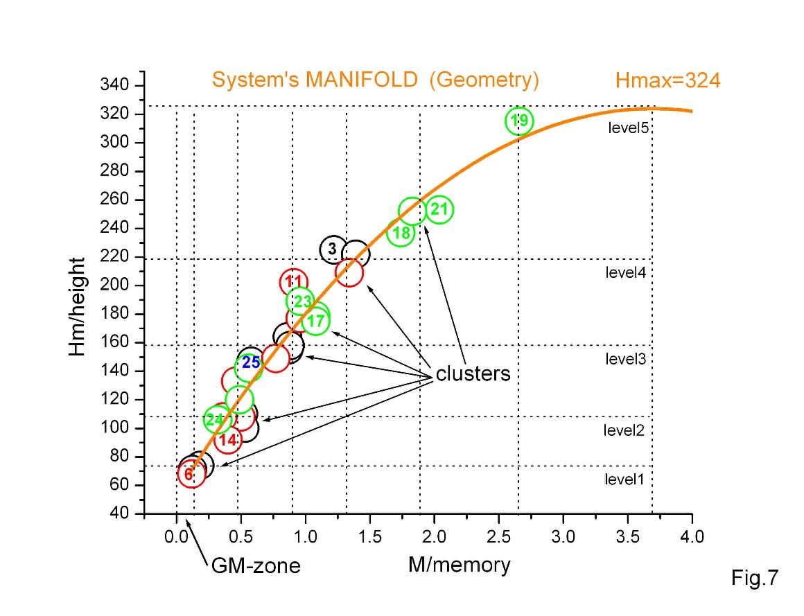
Figure 7. Manifold structure in (M, Hm) space: Geometric layer. To characterize the energetic state of the system, we introduce a memory parameter M, interpreted as a proxy for the magnetic energy accumulated in the solar convective zone. Motivated by the quadratic dependence of magnetic energy on field strength, we define: M ∼ ∫ SSN²(t) dt. In practice, this quantity can be approximated using cycle-level measures, but its conceptual role is that of an energy-like variable associated with the toroidal magnetic field. X-axis: M in the range 0–4; Y-axis: Hm in the range 40–340. Three Gleissberg-like (GL) cycles are shown: GL1 (black), GL2 (red), and GL3 (green). Individual Schwabe cycles (S-cycles) are represented by circles labeled by cycle number.
The system’s manifold is shown by the orange curve and has a quadratic form: Hm=53.8(±7.9) + 146.3(±14.9) •M - 19.8(±5.7) •(M^2) с H max=324 at M=3.7. Arrows indicate clustering structure and the transition region associated with grand minima (GM zone). In this region, M < 0.1 and Hm< 54. This threshold follows from the empirical correlation Hb ~ 54 + 0.28• Hp, where Hb and Hp denote the background and peak components in the SG3 decomposition. The resulting distribution of points reveals a well-defined, continuous structure rather than a scattered cloud. This indicates that the amplitudes of solar cycles are not independent but are constrained by an underlying relation with the system’s energetic state.
This figure represents the geometric projection of the system’s self-organization. The existence of a well-defined manifold indicates that solar activity is constrained to a low-dimensional set of admissible states determined by the system’s internal dynamics. Clustering along the manifold reflects preferred structural configurations, while the GM zone marks a limiting regime where coherence is reduced but not lost. Thus, the manifold encodes the constraints imposed by self-organization, defining the accessible states of the system. So, Fig. 1 provides a geometric representation of the continuous component of the dynamics, while the full behavior of the system emerges from the interplay between this constrained manifold and the discrete transitions discussed below.
SGK - hypothesis.
The present work is primarily devoted to a morphological analysis of solar activity in its minimal observational representation (the SSN time series). The results are interpreted within the framework of the SGK hypothesis, which views solar activity as a self-organized system whose behavior manifests through the Gleissberg cycle (GL-cycle), characterized by a well-defined structure of four pairs of solar cycles (11-year S-cycles). This structure is shaped by the centennial-scale MEC wave in the overshoot layer of the solar convection zone (SCZ).
The Schwabe–Gleissberg Knotting (SGK) hypothesis provides a structural reinterpretation of the centennial-scale variability of solar activity by identifying a previously unrecognized, internally constrained architecture of Schwabe-cycle sequencing. Instead of treating the Gleissberg cycle (GL-cycle) as a continuous or stochastic amplitude modulation, SGK demonstrates that its century-scale evolution follows a discrete, topologically restricted pattern enforced by the nonlinear dynamics of the solar convection zone.
Central to the hypothesis is the finding that each GL- cycle is composed of a fixed sequence of four pairs of Schwabe cycles (H-pairs), arranged in a characteristic pattern (Hs↑ → {H₂, H₃} → Hl↓) that persists across the entire historical record, including intervals following grand minima. SGK further shows that not all combinatorially possible morphotype transitions occur: the system occupies only a narrow, dynamically permissible subset of states. These restrictions arise naturally from Lorentz-force feedback, time-delay coupling between toroidal-field accumulation and meridional-flow adjustment, and inertia of deep-seated MHD flows, which jointly impose selection rules on permissible transitions between MA-types.
The hypothesis introduces the Magneto-Energetic Control (MEC) wave as the slow, physically grounded driver that modulates the accessibility of these states. Acting on century-long timescales, the MCE - wave governs the switching between H-pair types and generates the characteristic two-humped structure of the GL- cycle without resorting to phenomenological smoothing or purely statistical modulation.
Collectively, the SGK hypothesis establishes a unified dynamical picture in which the Gleissberg cycle emerges from the interaction of slow magneto-convective forcing with a discretely structured, topologically constrained configuration space of the solar cycle. This framework explains the invariant four-pair architecture, the asymmetry of early and late GL- cycle phases, the behavior of post-minimum recovery sequences, and the absence of forbidden morphotype transitions, thereby providing a cohesive structural basis for century-scale solar variability.
Theorem (Structural Invariants of the Gleissberg Cycle)
Within the framework of the three - loop MHD machine of the solar convection zone, the Gleissberg cycle possesses a set of topological and dynamical invariants. In solar activity dynamics, paired structures of Schwabe cycles (H-pairs) dominate over single S-cycles, reflecting the intrinsic inertia of MHD processes in the SCZ. 1. Pair structure. Each GL-cycle consists of exactly four H-pairs of Schwabe cycles: GL = [Hs↑ → {H₂, H₃} → Hl↓], where (Hs↑) denotes the first short rising pair, (Hl↓) the last long declining pair and {H₂, H₃} - second and third inner pairs.
2. Boundary stability. The first pair is always of type Hs↑, and the last pair is always of type Hl↓. These two boundary H-pairs are structurally stable invariants of the GL-cycle.
3. Internal configurational freedom. The second and third H-pairs admit, in principle, four formal permutations:
- H₂= Hs↑- MA4 - H₃= Hs↑
2. H₂= Hs↑ & H₃= Hl↓
3. H₂= Hl↓ & H₃= Hs↑
4. H₂= Hl↓ & H₃= Hl↓
4. Dynamical selection rules. Among these permutations, the configurations 2 & 3 are dynamically forbidden and are not observed in the empirical record. Thus, the observed GL-cycles represent a restricted subset of the formally allowed combinatorial space, selected by nonlinear MHD feedback and intrinsic time delays.
5. Saddle-cycle insertion. Adjacent H-pairs may be separated by a single MA4-type S-cycle, reflecting a transitional dynamo regime between two paired states. This insertion does not violate the four-pair invariant of the GL-cycle.
Physical Interpretation. The theorem implies that the Gleissberg cycle is not merely a loose centennial modulation, but a topologically constrained composite object constructed from four H-pairs of Schwabe cycles.
- The first Hs↑-pair corresponds to the growth phase of the MEC-wave under weak Lorentz feedback.
- The last Hl↓-pair represents the decay phase under dominant magnetic back-reaction and enhanced dissipation.
- The two middle pairs encode the nonlinear adjustment of the αΩ/BL dynamo to the slowly varying MEC background.
- The dynamically forbidden permutation (Hs↑ - Hl↓) results from magnetic quenching of meridional circulation and the α-effect by an excessively strong toroidal field (Lorentz back-reaction).
- The permutation (Hl↓ - Hs↑) is prohibited by the combined effects of flow inertia (time delays) and Lorentz feedback.
Hence, the GL-cycle emerges as a dynamically selected knotting of Schwabe cycles, rather than as a purely statistical centennial oscillation. In this sense, the Gleissberg cycle represents an emergent topological invariant of the solar dynamo rather than a phenomenological modulation of cycle amplitudes. In essence, each hump of the Gleissberg cycle represents an attempt of toroidal magnetic field (TMF) amplification driven by the growth phase of the MCE - wave but subsequently constrained by the LF-modulator (Lorentz feedback). After the first hump, the system enters a contradictory regime: the MCE-wave approaches its maximum, so the TMF retains a tendency toward further amplification despite the increasing pressure of the LF-modulator. As a result, solar activity remains at a moderately high level, while inertial forces—the TD-modulator (time delay)—prepare the formation of the next, third H-pair of the GL-cycle. The key question is the type of this emerging pair. Observations reveal three possible realizations: Hs↑{MA2.2–2.3} in GL1, Hs↑{MA2.3–2.3} in GL3, and Hl↓{MA3.1–3.2} in GL2. This implies that regrowth typically resumes as an Hs↑-pair after a single saddle-type SA4 cycle (#1 and #20) but may take the form of an Hl↓-pair {#11–12} after MA4 (#10). This behavior is directly controlled by the time available for energy accumulation in the third H-pair: in the first two cases, a full S-cycle is available, whereas in the third case the transition is effectively instantaneous. This is precisely how the TD-modulator manifests itself. The evolution of solar activity during the second hump of the GL2-cycle is particularly striking. After the first long and high S-cycle of type MA3.1 (#11; Fig. 2A), a sharp decline of the TMF occurs, followed by a transition to type MA3.2 (#12). At first glance, this might suggest the termination of the GL2-cycle. However, the structural constraints prove to be stronger than the local dynamics: a subsequent transition MA3.2 (#12) → MA4 (#13*) occurs with a maximal modulation parameter ε = 2. Cycle #13 is in fact long, although not as high as required for the first S-cycle of the final Hl↓-pair {MA3.1–3.2} (#13–14). Nevertheless, the GL2-cycle preserves its four-pair (4×H-pair) structure.
Hard distinction of the SGK-hypothesis from standard modulation paradigms.
All standard Gleissberg-cycle interpretations reduce the centennial variability of solar activity to continuous modulation of a single oscillatory dynamo mode—whether by stochastic forcing, weak nonlinear quenching, or linear superposition of multiple frequencies. The SGK-hypothesis is fundamentally incompatible with this class of models. It asserts that the solar dynamo operating in the convection zone is a multistable nonlinear MHD system with a discrete set of coexisting Schwabe-cycle morphological attractors, whose centennial organization is governed by their systematic knotting under the action of a slow MCE-wave. In this picture, the Gleissberg cycle is not an amplitude envelope but a topologically constrained sequence of attractor transitions, stabilized by Lorentz back-reaction and delayed flow response. The existence of H-pairs, forbidden permutations, boundary invariants, and saddle-cycle insertions implies that the centennial cycle possesses a discrete combinatorial skeleton, which is irreducible to any form of continuous or stochastic modulation. Consequently, SGK redefines the Gleissberg cycle from a statistical byproduct of fluctuations into a dynamically selected phase architecture of the solar dynamo itself. Thus, solar activity possesses self-organization and internal structure, because the following features are observed in it: 1. Stable attractors, 2. Formal structural units, 3. Nonlinear MHD feedback loops, 4. Hierarchy of time scales, (BHF), 5. Hidden slow driver (MCE), 6. Discrete morphological classes, 7. Noise resistance, 8. Strict transition rules, 9. Structural stability after extreme events, 10. Multistability of the phase space.
Now let's briefly describe the long-term MHD hierarchy of SCZ. The solar convection-zone MHD system operates in a self-organized, near-critical regime in which long-term modulation (the Gleissberg cycle) emerges as a structural invariant of the system rather than as an externally imposed oscillation. The Gleissberg cycle is the morphological footprint of a slow global energy cycle of the SCZ MHD system, manifested as the MEC-wave. The centennial MEC-wave can be described as a slow nonlinear relaxation mode of the solar convection zone, governed by the balance between convective energy input, magnetic dissipation, and Lorentz feedback. Its evolution modulates the effective α-effect and meridional circulation, thereby controlling the emergence, pairing, and suppression of Schwabe cycles. The MEC-wave represents a centennial-scale global energy modulation of the SCZ MHD system, acting in the overshoot layer and slowly reshaping the phase space of the solar dynamo. The observed diversity and sequencing of Schwabe cycles reflect the system’s trajectory through this time-dependent phase space.
Grand minimum corresponds to a global bifurcation of the solar dynamo system, in which the cyclic attractor governing Schwabe and Gleissberg variability is destroyed or rendered inaccessible, leading to a transition from a structured, modulated limit-cycle regime to a weak, non-cyclic deep dynamo state. The similarity between the characteristic durations of Gleissberg cycles and grand minima suggests that both phenomena are governed by the same centennial-scale reorganization of magnetic and kinetic energy in the solar convection zone. In this view, the MEC-wave represents a global relaxation process of the solar MHD system, whose active phase manifests as a structured Gleissberg cycle, while its suppressed phase corresponds to a grand minimum.
References:
Karak, B.B. "Models for the long-term variations of solar activity". Living Rev Sol Phys 20, 3 (2023)
Pesnell, W. D. (2016), Predictions of Solar Cycle 24: How are we doing? Space Weather, 14, 10–21, doi:10.1002/2015SW001304.