QTDE Approach to Long-Term Solar Activity
On Morphological Constraints and Competing Descriptions of Long-Term Solar Activity
Nick N. Kontor
Abstract
We present a low-dimensional morphological description of the historical sunspot-number (SSN) record spanning the period from approximately 1610 to the present. The analysis reveals a set of recurrent structural patterns, including paired solar cycles (H-pairs), isolated saddle-like cycles, and large-scale saddle regions associated with transitions between successive Gleissberg-scale states. The observed sequence of cycles appears to follow a restricted transition grammar characterized by discrete pathways, asymmetries, and apparently forbidden transitions.
These recurring structures suggest that long-term solar activity may not be adequately described as a sequence of independent cycles or stochastic fluctuations alone, but rather as the observable projection of an underlying dynamical organization possessing memory, recurrence, metastable states, and constrained transition pathways. Within this framework, solar activity can be interpreted as a partially self-organized multiscale system evolving on a low-dimensional state-space geometry.
The resulting morphology admits a structural forecast of the forthcoming Gleissberg cycle, including its expected sequence of solar-cycle states over approximately 9–10 Schwabe cycles.
We formulate this interpretation as a working hypothesis rather than a demonstrated theory. Its current limitations are threefold: (i) the absence of a generally accepted dynamical-systems description of the solar convection zone as a distributed dynamical system, (ii) the lack of a unique physical interpretation of the inferred morphological structures, and (iii) the absence of a rigorous quantitative assessment of the robustness and statistical significance of the proposed states and transition rules.
Nevertheless, the identified morphology suggests that long-term solar variability may be amenable to analysis within the framework of the qualitative theory of dynamical systems, where the primary objects of interest are not individual cycles themselves, but the invariant structures, transition pathways, and effective geometry governing their evolution.
Context and Motivation
The present work is motivated by developments in nonlinear dynamics, the qualitative theory of dynamical systems (QTDE), solar dynamo theory, and studies of long-term solar variability. Since the pioneering work of Henri Poincaré, qualitative approaches to complex systems have emphasized the importance of invariant structures, attractors, recurrence, bifurcations, and transition pathways rather than explicit analytical solutions. Similar ideas have subsequently appeared in nonlinear dynamics, state-space reconstruction, self-organization theory, multiscale systems, and modern studies of solar and stellar dynamos.
Despite substantial progress in solar dynamo modelling and MHD simulations, the long-term organization of solar activity remains only partially understood. The historical sunspot-number record exhibits both remarkable regularity and substantial variability, suggesting the coexistence of order and flexibility within the solar convection zone (SCZ). This raises a natural question: can long-term solar activity be described not only through physical mechanisms and numerical simulations, but also through the geometry and topology of its observable dynamical organization?
The present study explores this possibility through a low-dimensional morphological analysis of the historical SSN record.
Morphological Evidence
The proposed morphology is based on several recurrent structural features repeatedly observed throughout the historical sunspot record.
These include:
- H-pairs: recurrent pairing of consecutive Schwabe cycles into higher-order morphological units;
- MA classes: a finite set of recurring cycle morphologies;
- Λ-transition structures: preferred pathways linking successive morphological states;
- saddle cycles and saddle regions: transitional configurations separating different dynamical regimes;
- allowed and apparently forbidden transitions between morphological states.
Taken together, these features suggest that the observed sequence of solar cycles may not explore all possible configurations equally. Instead, the historical record appears to exhibit a restricted transition grammar characterized by recurrent states, preferred transitions, and persistent structural asymmetries.
This observation forms the central hypothesis of the present work. The hypothesis does not claim that the underlying physical mechanisms are presently known. Nor does it imply that the identified structures have yet been established as statistically rigorous dynamical invariants. Rather, it proposes that the morphology may represent a low-dimensional projection of deeper processes operating within the SCZ, thereby providing a candidate framework for investigating long-term solar activity from the perspective of qualitative dynamical systems theory.
INTRODUCTION.
The 11-year solar cycle is commonly interpreted as a self-sustained oscillation generated by the solar αΩ dynamo and often described in terms of a limit-cycle mechanism (Charbonneau, P., Sokoloff, D. 2023). Here I propose a somewhat different perspective, - not as an alternative to the dynamo framework, but as an attempt to describe the global dynamical context within which the dynamo operates, and thereby to render the picture more multidimensional. Solar activity, as recorded by the sunspot number (SSN), does not appear as a sequence of independent Schwabe cycles (here S-cycles) but rather as a coherent manifestation of a deeper, centennial-scale dynamical organization within the magnetohydrodynamic system of the solar convective zone (SCZ). Instead of treating individual cycles as isolated oscillatory events, this work approaches solar variability through the topology of phase space, viewing the observed cycle morphology as a trajectory constrained to a low-dimensional structure of a complex dissipative dynamical system (Guckenheimer & Holmes, 1983). This phase-space–topological framework provides a natural basis for interpreting long-term modulation and structural pairing of solar cycles as geometric properties of the underlying dynamical attractor, suggesting that the observed variability of the 11-year cycle reflects constraints imposed by the global structure of the dynamical system rather than stochastic fluctuations of individual cycles. This approach combines three main aspects of solar activity: physical, morphological and topological.
General theory of the solar interior (Christensen-Dalsgaard, 2021) identifies the solar convective zone (SCZ) as a complex dissipative MHD system, in which energy transported from the core through the radiative zone is converted into large-scale plasma motions and associated magnetic fields. From a physical standpoint, the magnetohydrodynamic (MHD) system of SCZ is described by plasma flows and magnetic fields defined at every point in space and time, making it an infinite-dimensional dynamical system. Such systems are governed by nonlinear partial differential equations (PDEs), and this mathematical framework constitutes the foundation of the αΩ-dynamo theory used to explain the 11-year solar (Schwabe) cycle (Charbonneau, 2020).
Within this framework, the Schwabe cycle (hereafter the S-cycle) is primarily shaped by several coupled physical processes: (f1) differential rotation generating toroidal magnetic field (Ω-effect), (f2) regeneration of poloidal field through cyclonic turbulence and flux emergence (α-effect / Babcock–Leighton mechanism), (f3) meridional circulation transporting magnetic flux, (f4) turbulent magnetic diffusion within the convective zone, and (f5) nonlinear saturation mechanisms limiting field growth. From a topological perspective adopted here, these processes act as fast variables governing the local oscillatory dynamics of the system. The morphological approach developed here does not replace this physical description but projects its high-dimensional dynamics onto a low-dimensional inertial manifold capturing the slow organization of solar activity.
Within this framework, solar-cycle morphology is introduced not merely as a descriptive classification but as a mathematical operation acting on time-series data. Strong temporal smoothing suppresses short-lived fluctuations and projects the sunspot-number signal onto its slow dynamical components, allowing each S-cycle to be represented by a reduced set of structural parameters describing its global shape. This operation effectively maps the original high-dimensional observational signal onto a low-dimensional phase-space representation, where individual S-cycles appear as discrete states constrained to a common geometric manifold. The resulting morphology therefore reflects intrinsic dynamical organization rather than observational variability, providing an empirical access to the underlying inertial structure governing long-term solar activity.
This follows from a meticulous morphological analysis of the accessible SSN time series (WDC-SILSO, Royal Observatory of Belgium), and also polar magnetic field (PMF) measurements, (dipole induction Avgf; Wilcox Solar Observatory), treated as reduced but dynamically meaningful projections of the magnetohydrodynamic processes operating in SCZ. So, this work is about how I understand now solar activity (SA), with which I have actually been dealing since the late 1960s. Technically, it consists of two parts: the first is "SSN time series SG - model", http://solarcycleforecastnnk.synthasite.com/, (2008-2020), the other is the one you are reading: "Solar activity prediction", https://solaractivityprediction.yolasite.com, (2020 - current). Both websites were written in real time, so they are unfinished and subject to constant revision. This is evident in their unstable structure. I apologize for this.
The SSN time series, derived from Wolf numbers, serves as the principal observational proxy of solar activity. Although it represents a severe dimensional reduction of a complex convective MHD system, it retains nontrivial structural information: nonlinear asymmetries, cycle-to-cycle coupling, multiscale modulation, and signatures consistent with self-organized behavior (Gershenson, C. 2025). A detailed morphological analysis of the smoothed solar cycle shape (SK-shape) described using a superposition of three Gaussian components (SG3 - model), demonstrates that while this representation successfully captures the internal structure of individual 11-year Schwabe cycles, it is insufficient to explain their long-term organization.
Solar magnetic fields are indirectly observed at the photosphere, most notably in the form of sunspots. R.Wolf proposed (1849) to quantify solar activity by sunspot counts, thereby introducing the sunspot number (SSN) time series. At present, SSN data exist in three principal forms, differing in temporal resolution and duration: daily data (D-data, since 1 January 1818), monthly data (M-data, since January 1749), and cosmogenic proxy records (C-data, e.g. ¹⁰Be and ¹⁴C isotopes (Usoskin, I.G. 2023)), which have a temporal resolution of the order of the solar cycle but extend over millennia. In the 1990s, I became interested in the observed shape of the solar cycle (S-cycle) and gradually developed a morphology of solar activity based on the M-data series, which contains three Gleissberg cycles (GL-cycles). The progress of this work is detailed on this website.
Morphological analysis reveals quite diverse features of solar activity in this SSN representation, a finite set of its stable states and a strictly constrained structure of transitions between them. Essentially, these observations are empirical constraints that any physical model of the solar convective zone (SCZ) must satisfy. They represent a certain structure of discovered facts, the physical connections between which remained unexplained until now.
Since the SCZ is a dissipative MHD system and therefore in principle (Nicolis, G. & Prigogine, I. 1977, Haken, H. 1983) capable of self-organization, its long-term evolution can be naturally described in terms of a structured phase space. We introduce the concept of Phase-Space Topology (PST) of the SCZ: a geometrically constrained organization of admissible trajectories that governs transitions between observable morphological states. In this framework, the empirically identified stable states correspond to dynamically preferred regions of phase space, while the observed transition rules reflect its topological structure. Within this approach, solar activity cycles are interpreted as trajectories evolving inside a slowly deforming phase-space topology, where morphological regularities emerge as macroscopic manifestations of underlying MHD dynamics. At the end of the text, a current long-term forecast of solar activity is examined
DATA PROCESSING.
M-data Strong Smoothing.
On my website (part_1), Fig. 9 shows how fragmented the available M-data is, not to mention the available D-data. It also shows the effect of smoothing (U-data). Another example is the available 13M-data, which is published alongside the available Y-data. The type of smoothing is critical to the task using SSN-data. The Fourier amplitude spectrum (FAS) of the available SSN-data reveals a dominant peak near 11 years, indicating the existence of a quasi-periodic solar cycle (S-cycle), along with several weaker spectral components. FAS has four (GL, S, Y, M/D) frequency ranges with the observable cutoff frequencies ~0.005 - 0.02 - 0.1 (1/month). It allows to get along with the observed SSN (monthly averaged M-data) the smoothed (by filtering) U-data (resolution ~5 months) and the heavily smoothed K-data (resolution ~2 years), see Figures 1, 3, 4, etc. The highest frequency included in the K-data is the second harmonic of the S-cycle, corresponding to a period of approximately 66 months. By choosing this cutoff frequency (0.02(1/month)) the SK-shape becomes smooth—free of visible peaks that correspond to fast processes such as stochastic turbulence, local SSN spikes, active-region outbursts, and quasi-biennial oscillations (QBO)—while still preserving the main Schwabe envelope (~11 years), the inherent S-cycle asymmetry (via retention of its second harmonic), and the centennial-scale modulation (the Gleissberg cycle).
The high-frequency filter functions as a local linear smoothing operator (SSO) performing a structural decomposition of the signal by extracting features that remain stable under rescaling and noise contamination. In terms of phase-space dynamics, this smoothing effectively projects the observed time series onto a low-dimensional inertial manifold (LDIM) capturing the essential slow dynamics of the system. According to Takens’ embedding theorem (Takens, F., 1981), the topology of the underlying deterministic attractor can be reconstructed from time-delayed observations, implying that the resulting SK-shape preserves the principal dynamical information despite the removal of fast fluctuations. Thus, the SSO with a cutoff period of approximately two years can be interpreted as an empirical projection onto the inertial manifold of the solar dynamical system. It suppresses fast αΩ-dynamo fluctuations while retaining the slow attractor geometry governing Schwabe- and Gleissberg-scale variability. Recovering the intrinsic morphology of individual S-cycles in this way enables a consistent parameterization of all 24 observed solar cycles.
At this point the analysis bifurcates into two complementary directions. The first, referred to as Morphological Solar Activity Analysis (MSA), proceeds toward the sections “The Current Conditions of Solar Activity and the Status of Their Prediction” and subsequently “What is the SG3-Model?”.
The second direction develops the framework of Dissipative Dynamical Systems Theory (DDST), which provides the theoretical basis for interpreting solar-activity morphology and its predictability. Within DDST, strong smoothing represents only the initial step toward identifying the low-dimensional structure of solar dynamics.
In schematic form, this hierarchy can be written as MHD PDE (SCZ)} > Dissipative semiflow > Global attractor > Spectral gap > Inertial manifold > Finite-dimensional ODE system > Hopf normal-form > Limit cycle. Our morphology is connected to this scheme via → projection to SSN(t) → strong smoothing operator (SSO) → SG3 morpho-structure. SG3 is the observed geometry of the normal form of its limit cycle in the SSN(t) coordinate. Thus, SG3 is an empirical representation of the limit cycle trajectory of the normal form in the SSN(t) coordinate, approximated by a superposition of three local amplitude wavelets. Or Normal form → Limit cycle in phase space → Projection onto the observed coordinate SSN(t) → Time parameterization of the cycle → Approximation of the form by three bell structures.
The primary structural feature of both the SSN morphology and the dynamical model of solar activity is the regular alternation of phases of growth and decline, realized through successive passages through extreme states. This conception is universal and will be used systematically henceforth.
The purpose of this work is to compare the results of solar activity morphology, represented by a series of SSN, with the ideas of dissipative dynamic systems theory (DDST), to formulate on this basis a hypothetical model of SCZ dynamics and to construct a long-term forecast of the Gleissberg cycle following from it.
The current conditions of solar activity and status of their short-term prediction are shown in figs.4, 4A, 4B and 4C. It is the chronicles of the constantly updated status of the solar cycle # 25 and a current status of # 26 forecast (fig.4C). This section examines current data of various types (M-, U-, K-data, PMF, PMF**) and their approximations, which are discussed from a purely morphological perspective. This allows one to become familiar with the solar activity data we are dealing with.

Figure 4 shows the current M-data, PMF-data, and K-data against the background of my forecast made in 2019 (25SGF, light gray). Initially, Hm was approximately 110, its refined value is 125±25 (see 25SGF revised, green). In essence, the forecast corresponded to the APM approach (see below, and also the APM's Contribution section). So, Figure 4 illustrates the evolution of cycle # 25. The interval [3205 – 3252] (months since January 1749) corresponds to the declining phase of cycle # 24, followed by the rise of S-cycle # 25. The reference forecast (light gray curve) is my (and approximately the same of NASA's) initial (2019) 25 - prediction, decomposed into three SG-components (thin curves). For comparison, three NASA's forecasts are also included (light gray). The highest forecast to date is the MT (Magnetic Terminator) forecast made by McIntosh, S.W., et al., 2020: 184±17 (see also Rodríguez, J., et al, 2024).
Our long-term forecast of solar activity begins with an initial prediction of the SK-shape of the future S-cycle. To realize this prediction, it is necessary to determine the expected type of the S-cycle (there are four in total), its cycle analogues, and its corresponding morphological attractor (the MA-cycle, of which nine kinds are distinguished). This proves possible within the TAA approach to the analysis of solar activity, which is based on our SGK hypothesis and the structural approach to the Gleissberg cycle derived from it (the GLS approach). All of this is described in detail below. But this is not the whole story. We must also estimate the expected amplitude of the S-cycle, Hm at t m, which is done using an adapted precursor method (the APM approach). It is precisely the combined use of these three approaches that makes our solar activity forecast especially detailed and, in a certain sense, unique. At the same time, this does not remove the fundamental limitation inherent in forecasting complex dynamical systems: uncertainty inevitably increases with time. As a result, initially our forecast was limited to one solar cycle ahead, with parameter uncertainties of up to ±20%. At that time, it seemed that this was the natural predictability horizon.
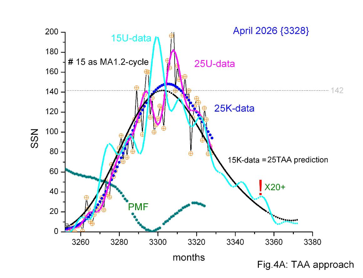
Figure 4A highlights the TAA approach: S-cycle # 25 is of the same type as S-cycle # 15 (MA1.2-cycle), which acts as both an analogue and a current attractor. The data already shown in Figure 4 have been supplemented with U-data for both S-cycles. It can be seen that from the beginning up to the maximum, S-cycles #15 and #25 proceed almost identically, although the U-data do not coincide. The difference in Hm is insignificant. Now the main interest lies in the difference in the decay phases of the cycles and the occurrence of the X20+ flare in cycle # 25. So far, the strength of the flares in it has not exceeded X9.
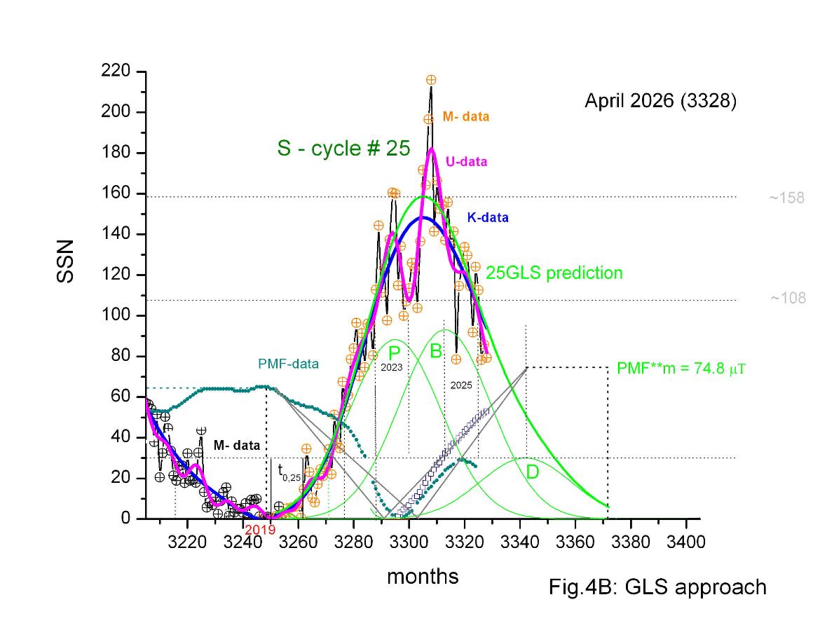
Figure 4B shows the consequences of the GLS approach. From Figure 2B, it can be seen that #25 has the form MA1.2, i.e., HA m = 158±18. It should be short with To = 120±6 months. As its SK-shape, we consider the parameters of the SG3-model for #15 (see Table 2). We estimate the moment of polarity reversal t pr = (Xp+t m)/2 = 3297 (this turns out to be practically accurate). The decay phase of the PMF (after its maximum in cycle #24) is described roughlyby a triangle with a vertex at point (3252/65) and the opposite side (3291.4-3303). The 25GLS prediction (green) represents a 15SK-shape with a corrected Hm*=158±18. This represents a certain average fundamental height, below which lie low and critically low S-cycles, while above it lie high and very high cycles. From Fig. 4 we get Hm** = 125±25, and from Fig. 4A - Hm*** = 142. The closest of these are the 25TAA prediction/142 (-3%), and also the 25GLS prediction/158 (+8%). The 25SGF revised is already underestimated by -15%, but all of them are within ±20%. A clear discrepancy is visible between the current PMF**(t) & PMF(t).
Now we can present a complete picture of the forecast for the next (currently # 26) S-cycle (see Figure 4C). We start with the GLS approach: what type and kind of cycle is expected? As for # 26, it appears to belong to type 2, i.e., a short, paired cycle, the first member of the Hs⬆️-pair (26-27). It is of kind MA2.1 (low, see Tables 2 and 3). The estimate for t pr is ~ 47.95 (3420). From this, the estimates are for 26PMF**m ~ 67 μT and 27Hm+ = 1.925 • 67 = 129. To obtain MA2.2, ε needs to be ~158/129 = 1.23, and to obtain MA2.3, ε needs to be ~218/129 = 1.69. In the first case, this corresponds to regime Λ₂; in the second, to regime Λ₃ (see table 3). According to approaches TAA and GLS, it should be expected that # 27 will be of the MA2.2 type, and the next Gleissberg cycle will have the configuration D2: Hs-Hs-MA4-Hs-Hl. How should we interpret this? We see that the structural forecast depends heavily on the specific values of the parameters obtained, the error of which we estimate as ±20%. Therefore, the forecast should be regarded as a baseline scenario, grounded specifically in the assumption regarding the adaptive nature of solar activity. The nature of the current development of solar activity is understandable and does not contradict the approaches considered, however, the available data do not yet allow for a confident and pretty precise long - term forecast of solar activity.
Comments to the current solar activity phase (years 2019 -2025 are now of only historical interest).
2019 (3241 - 3252): Solar monitoring showed that the first active region of the new S-cycle # 25 (AR2744) appeared in July 2019 (3247). After that, the stage of determining of the S-cycle # 25 start began, which lasted a whole year and showed that S-cycle # 25 actually began in November 2019 (3251), but according to M13-data - in December 2019 (3252). S-cycle #24 actually ended in April 2020 (3256).
2020 (3253 - 3264): It is the first year of S-cycle # 25 which was developing at that time in the mGM stage (3215 - to,25 (3252) - 3271). Having 25SGF, it is possible to evaluate the year averaged SSN (Y*-data= 13 ± 5.3) and compare it with observations (Y-data=8.8±4.1). It is seen (see also figs 4) that activity is low (less than one sunspot on the visible photosphere) and changes by an unpredictable way. Nevertheless, it can be seen some M-peak in November which penetrates in the active zone (M-data = 34.5±8.1).
2021 (3265 - 3276): This year, M-data grew steadily and after 3271 was already in the active zone. Y-data showed this: Y*-data = 39.7 ± 10.6 and Y-data = 29.6 ± 7.9. An abrupt increase in activity is also shown by M-peaks in September (M-data = 51.3 ± 9.6) and in December (67.5 ± 15.6). Thus, in August 2021, the mGM-period ended and the fast growth phase of S-cycle # 25 began.
2022 (3277 - 3288): The growth in activity continued throughout the year, in May M-peak was noticeable (M-data = 96.5 ± 16.3), and in December the activity level was twice as high as in January 2022. U-data allow us to clarify the course of M-data, showing its fluctuations with period of the order of a year. Formula (1) can now be written as follows: M-data ± σm = U-data ±<σu> (1), where σm is the observational error of M-data and <σu> =17 is the mean deviation of M-data from U -data (see Figure 9). The first three years of cycle #25 can be tentatively described by the SG(n)-model with n=4.
#1: 3256 - 4.37 - 3.6
#2: 3265 - 7.23 - 18.3
#3: 3278 - 9.86 - 49
#4: 3292 - 14.81 - 113
The current U-curve, currently described by n U-peaks, changes markedly as new M-data arrive. In this case, only U peaks with numbers < n-3 are more or less stable. In other words, you can always adjust U-data by U-peaks, but the U-shape will take on its final form only at the very end of the S-cycle. The situation is as follows: K-data describe the almost regular effects of the S-cycle (its growth, maximum activity and its decline) in the form of its P-, B- and D-components; their features are seen on the scale of centuries in the form of Gleissberg cycles. U-data show already the details of the noted effects, appearing in the form of U-peaks. U-data are sensitive to unpredictable abrupt changes in M-data, so their prediction cannot be justified right now. On the other hand, U-data can carry information about the features of the shape of S-cycles, but this issue requires a special study. The whole of 2022 (as well as the second half of 2021) falls on the solar activity's growth phase in S-cycle # 25. In December, exactly three years after the start of S-cycle # 25, M-data reached the level of the predicted maximum of the cycle (Hm=110). Figures 4 show that K-forecast (25SGF) matches the behavior of M-data quite well throughout this period.
2023 (3289 - 3300): In January, M-data reached the current high of 143.6 ± 29.2, and for the first five months of this year, the average <M-data/5> was 122.3 ± 19.4, which is very close to the prediction of Hm+,25= 126 ± 3 (given by Pawan Kumar et al. in ApJ 909:87, 2021 March 1). Having completed the forecast of the course of SA for the next ~100 years, we can again move on to pressing matters, namely worries about maximum # 25, which may happen soon in several months. There are now at least two fresh forecasts - besides mine (110± 8) - Kumar et al, 2021 (126± 3) and NOAA at 10/19/2023 (155±18 between January and October 2024). Let's move on to the process of estimating Hm (#25) from current K-data. According to data from 3296 (August 2023), we obtain Hm=121 at t m= 3302, February 2024, which is 10% higher than 25SGF. Data for September (3297) give Hm, k = 131 at 3303 and for October - 112 at 3298. Summary for November 2023: we observe the first sU-peak of the S-cycle # 25 (Hm=139 at 3294, June 2023, compare with fig.3); moreover, the maximum of the predicted P-component falls on 3290 (February 2023). For K-data the maximum is 115 at 3299 (see figs 4). t pr has still not arrived and now is six months behind my forecast (3293).
2024 (3301 - 3312). In January it became known that t pr = 3296 (August 2023). This allows you to begin comparing the observed PMF(t) with the calculated PMF**(t) in real time (see Fig. 4). Regarding Hm (t m), to what was said about the last three forecasts (2019, 2021 and 2023) above (see comment for 2023), we can add that Y -data (2023) = 125.3± 19.2, and this is today makes the 2021 forecast a favorite. As for my 2019 forecast, I am inclined to estimate the error in determining the value of any parameter of the SG - model as σ*= (15±5) %. It is interesting to note that based on the estimate t p = (Xp+t m)/2, we get t m = 3301 or January 2024, which means that the maximum of S-cycle #25 is somewhere nearby.
Be that as it may, over the course of 16 months (January 2023 - April 2024), M-data fluctuated at a 'quite acceptable' level of 124.6±19.7. During this time, a small sU1-peak = 140.4 at 3294 (June 2023) was observed. However, starting in May 2024, M-data began to rise rapidly, leading in August to the current observation (based on K-data) of Hm=190.8 at 3318, which corresponds to June 2025 (in April it was 126.5 at 3303, in May already 154.9 at 3312). Accordingly, based on U-data, we have sU2-peak = 213.7 at 3310. Obviously, this significantly exceeds all forecasts. However, what the actual sU2-peak and 25Hm (t m) will be, we still have yet to find out. For now, considering the latest adjustments, we get 25Hm*= 65 (24PMFm) •1.925 (±0.147) ~ 125 ±10. This means that soon we should expect the end of the sU2-peak and the beginning of the decline phase of S-cycle # 25. Moreover (see below), considering that S-cycles # 15 and 25 are analogs, a Super flare of class X20 or higher can be expected in the period 2024-2027.
As of September 2024, Figure 4A shows that the growth phases #15 and #25 (the first three years) in K-data are similar, but initially, #25 K-data trends lower and then surpasses #15 K-data near the peak (for now). The U-data shows greater divergence: first, a #15U peak appears, followed by #25U, #15U, and #25U. At this point, the peak phase ends, but 25Hm(t m) remains unknown. Overall, #25 lags slightly behind #15. Now about the super flares. In #15, they occurred around 6.1921±1 month. If the peak of #25 is around 6.2024, a super flare of class X20+ could happen in the summer of 2028 (3306+48=3354). A significant marker (!) is placed there. The first comparison focuses on U-data as the most sensitive smoothed data. U-data is primarily characterized by super peaks (sUi). For #15, these are sU1 (3275), sU2 (3299), the primary peak; smaller ones include sU3 (3322), sU4 (3342), and the final one, sU5 (3354), during which the X20+ super flare occurred. For #25, so far, there are sU1 (3294) and sU2 (~3307), the main peak. We observe that the positions of sU peaks do not align; however, the primary sU2 peaks are quite close, but it is too early to speculate on their total number. The general conclusion is that neither M-data nor U-data allow for a long-term, accurate forecast. Moving on to K-data, they follow a steeper trend than curve #15: at 3284, they intersect 25SGF*, and at 3299, they cross the 15SK-shape. The situation remains uncertain and critical for the APM forecast, though still within the bounds of previous predictions, as seen in Figure 4. It should be noted that Figure 4 presents the 25SGF19 forecast, representing the 25SK-shape forecast (thick green), reflecting my knowledge as of 2019. The data in Table 2 are treated as initial values for fine-tuning the 25SK-shape using the SG3 model. In addition to SSN, super flares of class X20+ were also considered. The results indicate that during the decline phase of #25 (between 2024–2028), despite relatively low activity, such a flare is possible. By the way, on October 3, 2024, a class X9 flare was recorded. Will there be a super flare in the current cycle?
Super flares as a Marker of Saddle S-Cycles. Here is a list of events accompanied by X20+ class flares:
1. Carrington Event – September 1–2, 1859. The equivalent class is possibly X45. It was S-cycle # 10, t m ±1 year.
2. Geomagnetic storm of February 4, 1872? This event was likely related to a powerful solar flare, but specific data on its strength is unavailable. It is S-cycle #11, t m +1 year.
3. Flare of May 14–15, 1921. Although the exact strength of the flare is unknown, its impact suggests it could have been an event of X20 or greater magnitude. Flare of July 23, 1921. This event caused powerful auroras and disruptions in telegraph systems. It is possible that it was also an X20 or higher-level event. This is S-cycle # 15, t m+ 4 years.
4. Flare of November 12, 1960, possibly reaching X20 level. S-cycle # 19, t m + 2 years.
5. Flare of August 4–7, 1972. This series of flares included one powerful flare (possibly X15 or higher). S-cycle # 20, t m + 4 years.
6. Flare of March 6–10, 1989. Although the strength of this flare was below X20, its effects were catastrophic. Flare of August 16, 1989 (X20):Occurred in active region AR 6659. This event also triggered strong geomagnetic storms on Earth. Flare of October 19, 1989 (X13). S-cycle # 22, t m ± 1 year.
7. Flare of April 2, 2001 (X20): Occurred in active region AR 9393. This is one of the strongest flares in recent decades. Flare of October 28, 2003 (X17.2). Flare of November 4, 2003: Initially estimated at X28, but the actual strength may have been up to X45 (due to instrument saturation). Flare of September 7, 2005 (X17). S-cycle #23, (t m + 2) ± 2 years.
Of the 7 proposed super flares, all of them occurred within the period (t m + 2) ± 2 years in S-cycles # 10, 11, 15, 19, 20, 22, 23. This leads us to conclude the following: Super flares occur in high cycles with a probability of ~80%, and in low cycles with a probability of ~20%. Super flares arise at the beginning of the declining phase of the S-cycle, within the period (t m + 2) ± 2 years. According to the SG3-model, super flares occur during the maximum of the B-component and may be associated with the second sU-peak in U-data. Super flares appear (in our example, with 100% certainty) in higher members of the H-pairs and in saddle cycles (#10, 15, 20), which are significantly lower. Therefore, the likelihood of a super flare in cycle #25 is high.
2025 (3313–3324). The period from August 2024 (when M-data(t) peaked at 216 on at 3308) to May 2025 (when M-data(t) sharply declined to ~80 at 3317), lasting nearly a year, can be regarded as the second phase of the maximum of Solar Cycle 25. The first phase had occurred from December 2022 to August 2024, i.e., for more than a year and a half. This asymmetry in the maximum phases is due to the unexpected sU-peak, whose height was ~214 at 3310 (based on U-data). The end of the second phase—when M-data consistently remains below 100—is still uncertain. However, as of May 2025, M-data has declined significantly, reaching values substantially lower than during the Cycle 25 maximum. For example, in April, the current 25Hm* was ~150 at 3309, clearly exceeding my forecast corridor: {Hm⁺ = PMFm (±5%) • 1.25 (±0.05) • 1.54 (±0.12) = PMFm • 1.925 (±10.1%)}, and assuming 24PMFm = 65 μT, the expected 25Hm = 125.125 ± 12.638, with the 1σ upper bound = 137.763. But in May, 25Hm* dropped to ~144 at 3303. From this point, M-data is expected to gradually decline, eventually leading to a “final” value of 25Hm. Although the precise final value is currently unknown, we can estimate a lower bound of 25Hm(min) ~145 at 3300, assuming that M-data becomes zero after May and remains so until the end of 2025. This suggests that the final 25Hm will likely be ~145, which places it near the lower edge of NASA’s forecast corridor (as of 2023/10/19), while my own forecast will be underestimated by approximately 2σ, or ~20%. Figure 4A shows that, so far, the 25SK-shape almost perfectly replicates that of S-cycle # 15.
In August (3320), 25Hm = 147.2 at 3308. The cycle is undergoing a transition from the maximum phase to the decline phase. The beginning of a new (seventh) U-peak can be seen. In Figure 4A, it is evident that cycle #25 lags somewhat behind its analogue/attractor SA1.2 (#15). Otherwise, their SK-shapes are quite similar. It is worth noting that so far PMF(t) and PMF**(t) have been almost identical, which suggests ε ~ 1. If this situation persists until the end of #25, it will serve as independent confirmation of the onset of the first regular Hs⬆️-pair (#26–27) of the new GL4-cycle.
As of December 2025 (3324), the following changes in the situation can be noted. The observed height is 25Hm, c ~146 at 3307, i.e., it has more or less stabilized at a moderately high level (158±18). However, the declining phase of the cycle is apparently being slowed down by a new U-peak. As for the course of PMF, a discrepancy between observations and PMF**(t) has emerged.
2026 (3325 - 36). Figures 4, 4A, 4B and 4C illustrate the current period of solar activity (M-data and PMF-data), analyzed from three complementary predictive perspectives: APM, TAA, and GLS.
APM is a widely used linear precursor method, according to which the value of PMFₘ during the declining phase of an S-cycle determines the amplitude (Hₘ⁺) of the subsequent S-cycle. In this work, we employ the regression Hₘ⁺ = 1.925 · PMFₘ (±20%). The APM approach is effectively illustrated in Fig. 4 and, in essence, assumes the stability of the S-cycle dynamo mechanism. From the standpoint of morphological analysis of solar activity, a key limitation of APM is the difficulty of reliably estimating PMFₘ for any S-cycle, whether past or future. The TAA approach follows from the observation that, although S-cycles differ from one another, the nature of these differences is not arbitrary. Distinct types of S-cycles, their analogs, and possibly even morphological attractors can be identified. This approach is illustrated in Fig. 4A. The abbreviation GLS reflects the concept that the Gleissberg cycle possesses an intrinsic structure, meaning that the evolution of S-cycles is governed by the internal dynamics of the MHD system of the solar convective zone (SCZ). From a morphological perspective, this manifests as the discreteness of the principal S-cycle parameters. The structure of the GL-cycle defines a discrete set of allowable parameter values for the S-cycles composing it, while stochastic forcing broadens these values within ±20%. The GLS approach encompasses both the TAA and APM frameworks, as shown in Fig. 4C.
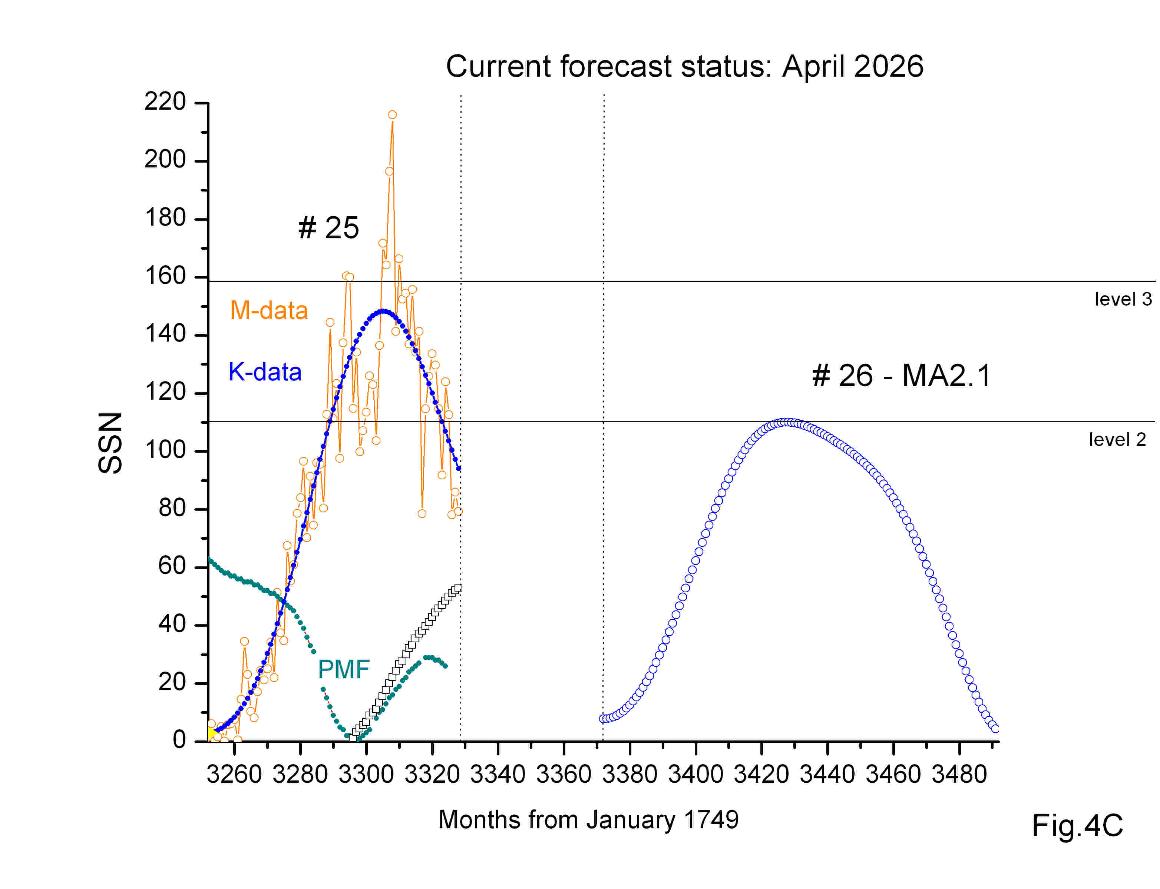
Let us examine the current state of solar activity (see Fig. 4C). As follows from Fig. 4, just before the onset of S-cycle #25, NASA/NOAA expected a peak amplitude of approximately 25Hₘ ≈ 115, while I, based on my APM at that time (with 24PMFₘ = 65 μT already known), obtained a value of about 110. Moreover, taking into account the mean parameters of low-amplitude short cycles—which is precisely how S-cycle #25 appeared at that time in the context of Fig. 2A—I adjusted the parameters of its SG3 model to these values (see 25SGF in Fig. 4). After the onset of S-cycle #25, two processes unfolded in parallel. First, NASA/NOAA incorporated newly accumulated cycle data into its ensemble forecast, which led to its revision in 2023 (the upward revision of the SC25 forecast reflects not a change in methodology, but the incorporation of early-cycle morphological constraints that were not available at the time of the original precursor-based prediction). Second, I continued my morphological analysis of solar activity, which by 2025 resulted in the GLS concept described on this website. This concept makes it possible, prior to the onset of the next S-cycle (now #26), to infer its expected type. Specifically, it is predicted to be a short, low-amplitude S-cycle of the second type, representing the first member of the first Hs⬆️-pair (#26–27) of the new GL4 cycle. This type corresponds to an MA2.1 cycle, i.e., a morphological attractor constructed from the analog cycles #7 and #16 (see Table 2 on p. 2 and the subsection “Main parameters of the 9 MA attractors” on p. 3). This MA-attractor is shown in Fig. 4C.
As for S-cycle #25, in hindsight it can be characterized as a single transitional short S-cycle of the first type, corresponding to an MA1.2 cycle, a morphological attractor whose prototype is cycle #15 (see Fig. 4A). The APM approach would yield 25Hₘ⁺ = 1.925 × 65 = 125.125, whereas H_Aₘ = 158 ± 18 (see Fig. 4). Already at present it can be stated that the actual peak amplitude 25Hₘ lies approximately midway between these two values. To estimate the height of S-cycle #26 using APM, we need to know 25PMFₘ. We take PMF**ₘ = 74 μT as a known value, since cycle #25 is of type MA1.2; a calculation based on my SGF2019 forecast yields 65 μT. A real-time comparison between observations and calculations is currently underway (with an accuracy of ΔT = (25T₀ − 3296)). As always, the ε-problem is also present.
As can be seen from Fig. 4C, three values are currently under consideration for the peak amplitude 26Hₘ: 108 (the “structural” value), and the APM-based estimates 26Hₘ⁺ = 1.925 × 74 = 142.45 or 1.925 × 65 = 125.125. The calculated values may be adjusted by the parameter ε, whereas actual measurements of 25PMFₘ, should they deviate significantly (by more than ±20%) from approximately 56 μT, would raise questions either about the APM approach or about the GLS framework itself.
We may now summarize what can be forecast and what can be monitored. Our morphological analysis suggests that solar activity is not a purely stochastic phenomenon, but is shaped by the self-organization of MHD processes in the solar convective zone (SCZ). This self-organized structure, however, is inherently imperfect: it is systematically blurred—typically within ±20%—by the intrinsic stochasticity of the same MHD processes that generate it.
This leads to a fundamental, semi-quantitative conclusion. The long-term evolution of solar activity is not random, and its qualitative modes of change are intelligible within the SGK hypothesis. At the same time, this intelligibility does not imply unlimited predictability. The solar dynamo appears to possess memory, but this memory is finite. As a result, the horizon of genuine predictability is effectively restricted to a single solar cycle. Beyond that horizon, determinism gives way to structured uncertainty: only alternative evolutionary scenarios can be meaningfully discussed, constrained within the framework of a single Gleissberg cycle.
The current situation can be summarized as follows. S-cycle #24 (type_3) has ended and can be fully described (see Table 2); it completes the GL3 cycle. The ongoing S-cycle #25 is transitional (type_1) between Gleissberg cycles. The predicted S-cycle #26 (type_2) will be the first S-cycle of the GL4 cycle, and at present nothing about it is known with certainty. What is essential for us is knowledge of the M-data, t₀, Xₚ, t_pr, tₘ and Hₘ, PMFₘ, T₀, as well as all parameters of the SG3 model of the S-cycle and the parameters of all U-cycles. This information allows a complete description of an S-cycle (as in the case of #24) and, partially (with the exception of PMFₘ for S-cycles earlier than #21), of all cycles starting from #1.
For S-cycle #25, as of today (December 2025), only M-data, t₀, t_pr, and PMF(t) are known. Its forecast was made in 2019 based on the APM available at that time, the known value 24PMFₘ = 65 μT, and the mean parameters of the SG3 model. In 2025, the SGK hypothesis was proposed, on the basis of which new APM, TAA, and GLS approaches to the analysis and forecasting of solar activity were developed. According to these approaches, the forecast for S-cycle #25 was refined: APM yields 25Hₘ = 125 ± 25, TAA gives 158 ± 18, 25PMF**ₘ = 65 μT, and T₀ = 120 months (±5%). During the declining phase of the cycle, an X20+ flare is expected. This forecast requires further verification through observations and data analysis.
For S-cycle #26, the GLS and TAA approaches determine its type, its attractor (MA2.1), and, consequently, 26Hₘ = 108 and 26PMF**ₘ ~ 61 μT. Moreover, the form of the SG3 model for MA2.1 is known, i.e., practically all key parameters. The values of t₀ and T₀ are known with an accuracy of ±6 months. The remaining question is how accurate these estimates will prove to be and whether the conditions of the SGK hypothesis will remain valid. From the APM perspective, 26Hₘ⁺ = 1.925 · PMFₘ = 158, 135, or 116. Our calculation of 25PMF**ₘ is performed under the assumption ΔT = 79 months and yields 65 μT. The value of T₀ may be 114, 120, or 126 months. This corresponds to ΔT = 70, 76, or 82 months, or PMF**ₘ ≈ 82.8, 70.2, or 60.3 μT. For our approach to be valid, ε must therefore be 56 / 82.8 = 0.68, 0.8, or 0.93, i.e., < 1. In other words, the observed PMF(t) must be lower than the calculated PMF**(t).
At present, we are refining the estimate of 25Hₘ, comparing observed and calculated PMF values, examining the correspondence between cycles #15 and #25, anticipating a super flare, and describing the overall forecast situation for S-cycle #26.
What is the SG3-Model?
The SSN time series can be presented as the dependence of the number of sunspots on the Sun over time (e.g., in the form of a table or graph) and at the same time as a Fourier amplitude spectrum (FAS), showing which frequencies (periods) are most clearly manifested in the SSN time series. At the very beginning, it became clear that the M-data exhibited excessive fluctuations and therefore needed to be smoothed (see Figs. 1, 3, 4). This is a common procedure (see, for example, the M13-data); however, the question is, what is the purpose of smoothing? My goal was a "good" description of the SSN-data, and the result of my strong smoothing (see above) fully satisfied this goal. The SK-shape of each smoothed S-cycle was described by the SG3-model, which was a superposition of three bell curves, i.e., SG3(t) = P (t, Xp, Ap, Wp) + B (t, Xb, Ab, Wb) + D (t, Xd, Ad, Wd). This function has 9 parameters, and each S-cycle described by it has 13 parameters (+ to, To, Hm at t m). Thus, the function SG3(t) is an S-cycle parameterization operator that transforms the point curve K(t) into a set of 13 numbers (see Table 2).
So, to recover the intrinsic shape of individual S-cycles, the original SSN time series was filtered to suppress high-frequency fluctuations. It allows reliable reconstruction of the shapes of the last 24 S -cycles. Each cycle shape (SK-shape) was approximated by an SG3-model, defined as a superposition of three Gaussian normal functions. As a result, each S-cycle is characterized by a set of 13 parameters, of which 9 are temporal and 4 are amplitude-related. This representation embeds each cycle as a point in a finite-dimensional parametric phase space. Description of the smooth K-shape of different observed S-cycles by many parameters (out of 13 parameters, the most meaningful changes occurred in the parameters: Xp, Hp, Hb (Hp), To, Hm (t m)) is achieved using W = 33 months and some masking of the S-cycle onset and termination, which yields χ² ≈ 0.1. The resulting database 13 x 24 (Table 2) provides a systematic record of variations in S-cycle morphology.
If the result of the first step of decomposition of observational data can be called phase-space morphological projection, which effectively projects the original time series onto a low-dimensional manifold representing the slow dynamics of the system, then the second step is morphological topologization, which converts each smooth SK-shape into a vector of 13 numerical parameters; encodes the morphological structure of the cycle into a feature space suitable for statistical analysis, regression, and phase-space trajectory reconstruction; prepares the data for building the multidimensional morphological figure and mapping its relation to the SCZ attractor.
Examination of the FAS form led to the identification of four frequency ranges within it. By filtering out the highest frequency range (M/D), we obtained the U-data, and by additionally filtering out Y-range, we obtained the K-data. The SG3-model for describing K-data was constructed intuitively, assuming that any SK-shape could be well described by the superposition of three bell curves with a "width" (4•σt) of approximately 66 months (the second harmonic of the S-cycle) and a half-width (W = 2•σt) of approximately 33 months. Fitting the SK-shapes for S-cycles ## 1 - 24 took a lot of time but eventually led to Table 2.
The SG3 - model suggests that the SK-shape is assembled from three components: P, B, and D, the emergence of which can be explained by changes in the properties of sunspot groups at high, medium, and low heliolatitudes. The magnetic structure of sunspot groups undergoes significant changes throughout the 11-year solar cycle, reflecting the changes in the global magnetic field. At the beginning of the cycle, spots appear at high latitudes (around 30° and above). These spots are usually small and have a simple magnetic structure. As the solar cycle approaches its maximum, the number of spots increases, and they begin to appear at lower latitudes (around 15-20°). The sunspot groups become more complex and larger. The magnetic fields in the sunspot groups also strengthen, leading to longer lifespans of the spots (this period of the cycle is described by the P-component).
During the period of maximum solar activity (described by the P - and B - components), spots appear at latitudes of 10-15°. The magnetic structure of sunspot groups becomes the most complex. In large sunspot groups, several pairs of spots with opposite polarity, aligned along the latitude line, can be observed. During this period ~ ((t m+2) ±2 years), powerful solar flares (class X20+) and coronal mass ejections occur in certain sunspot groups and S-cycles, associated with the redistribution of energy in complex magnetic structures. As activity decreases, spots appear at even lower latitudes (around 5-10°) and begin to shrink in size (the period of the D-component). The magnetic structure of the spots becomes simpler and less organized again, and the number of sunspot groups decreases. Thus, over the course of the S-cycle, sunspot groups progress from simple, small structures with disorganized magnetic fields to more complex and large structures with strong and organized magnetic fields and then simplify again towards the end of the cycle, as if preparing for the start of a new one. Using the SG-model, any S-cycle (## 1-25) can be described, in two forms - SK - & SU -shapes. Examples are in Fig. 1 (# 1), 3 (# 24), 4 (# 25).
SK-shape of any S-cycle can be written as G1+G2+G3, where the basic component of the SG-model has the form G i (t)= H i • exp {- 2 • [(t - X i) ^2]/ (W i (^2))}. Symbolically SG3-model can be written as: # S3 = to + Xp - Wp - Hp = + Xb - Wb - Hb (Hp) = + Xd - Wd - Hd = To = Hm at t m. It contains 13 terms that must be defined during fitting and specified during forecasting. Here to is the cycle start date (ordinal month, where January 1749 = 1), Xp,b,d are the moments of the component maximum, Wp,b,d = 33 months, Hp is the height of the first component, Hb ~ 54 + 0.28 • Hp (regression), Hd is the height of the third component. So, the SK-shape of S-cycles is well described by the superposition of three bell curves Gi (t, Xci, Wi , Ai), where i = 1, 2, 3 (P, B, D-components), Hi = Ai / {[( π/2) ^1/2] • Wi}, To is the cycle length, Hm at t m are the magnitude and time of the maximum, the results are shown in Table 2. Let's move on to the next page.
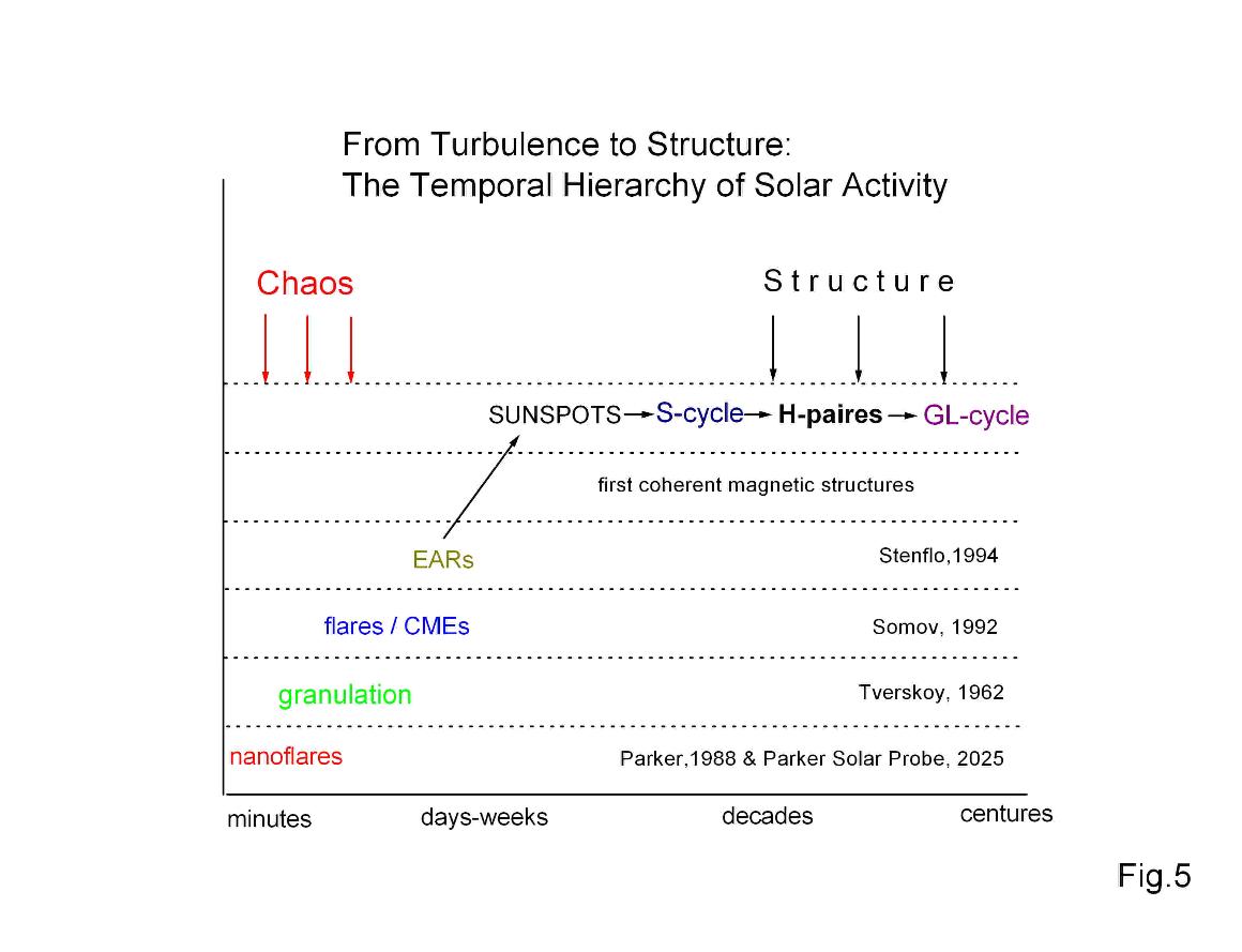
Figure 5 shows the principal manifestations of solar activity in relation to their characteristic timescales. Nanoflares, as one of the mechanisms of coronal heating, were introduced by Eugene N. Parker (1988) and subsequently supported by observations from the Parker Solar Probe. Granulation, as a manifestation of solar convection in the photosphere, generates small-scale background magnetic fields (Boris A. Tverskoy, 1962). Solar flares and coronal mass ejections (CMEs) arise from large-scale magnetic reconnection processes in the solar atmosphere (Boris V. Somov, 1992). Ephemeral Active Regions (EARs) serve as tracers of large-scale magnetic fields and provide evidence for magnetic coupling between neighboring solar cycles (N. N. Kontor & T. G. Khotilovskaya, 1988; Scott W. McIntosh et al., 2020). Sunspots represent the most recognizable “symbols” of solar activity; their number (Rudolf Wolf, 1848) follows the law of the solar cycle (Heinrich Schwabe, 1843).
All these phenomena possess their own internal structure and dynamics, which define their identity, their role in solar activity, and their place in solar physics. Our goal, however, is to identify a global, long-lived structure of solar activity that governs its long-term variability—that is, the variability from one solar cycle to the next. As it turns out, such a structure most likely exists, but its fundamental unit is not the Schwabe (S) cycle itself, but rather an H-pair of coupled S-cycles. The concept of paired S-cycles is not new: it was discussed by George Ellery Hale (1924) in the context of magnetic polarity reversal, and by M. N. Gnevyshev and A. I. Ohl (1948) in the form of the Gnevyshev–Ohl rule. However, our H-pair is a dynamical unit associated with the regime of meridional circulation (MC) and, more generally, with the instantaneous MHD state of the entire solar convection zone (SCZ). H-pairs exist in two forms (see Figure 6), and it is precisely their alternation—occasionally interrupted by the appearance of isolated S-cycles—that gives rise to the observed long-term variability of solar activity in the form of the Gleissberg cycle.
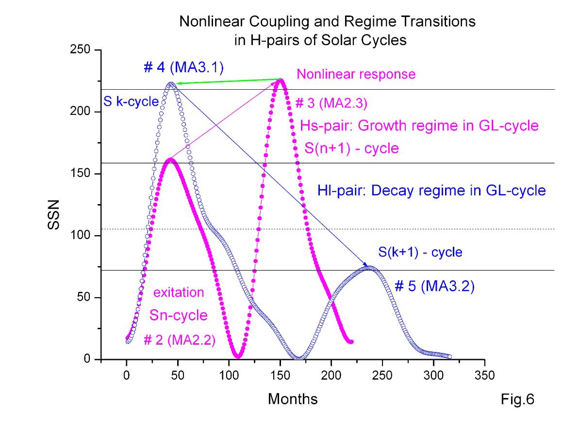
Figure 6 illustrates examples of both types of H-pairs. Magenta represents a short, ascending pair of type Hs⬆️—specifically, S-cycles #2 and #3. Upon its completion, a transition occurs (indicated by the green arrow) to a long, descending pair of type Hl⬇️, comprising S-cycles #4 and #5. For ease of comparison, the starting points of the pairs have been aligned. It is evident that during the transition between these pairs (see Fig. 2B), the amplitude of the S-cycles (specifically #3 and #4) changes only slightly; however, the cycles within the new pair become longer, and their morphology undergoes a substantial transformation. In this particular example, the duration of the pairs differs significantly: the Hs-pair spans 220 months, whereas the Hl-pair lasts 315 months. This suggests that the dynamic regimes governing these pairs are markedly distinct.
References:
Charbonneau, P., Sokoloff, D. Evolution of Solar and Stellar Dynamo Theory. Space Sci Rev 219, 35 (2023). https://doi.org/10.1007/s11214-023-00980-0
Charbonneau, P. Dynamo Models of the Solar Cycle. Living Reviews in Solar Physics, 17, 4, 2020
Christensen-Dalsgaard, J. “Solar structure and evolution”, Living Reviews in Solar Physics 18, 2 (2021)
Gershenson, C. "Self-organizing systems: what, how, and why?" npj Complexity 2, 10 (2025)
Gleissberg, W. "The secular variation of solar activity". Journal of Geophysical Research, 44, (1939)
Guckenheimer, John & Philip Holmes, “Nonlinear Oscillations, Dynamical Systems, and Bifurcations of Vector Fields”, Springer, 1983
Haken, H. "Synergetics: An Introduction. Non-equilibrium Phase Transitions and Self-Organization in Physics, Chemistry and Biology", Springer (3rd ed. 1983)
McIntosh, S.W., Chapman, S., Leamon, R.J. et al., "Overlapping Magnetic Activity Cycles and the Sunspot Number: Forecasting Sunspot Cycle 25 Amplitude". Sol Phys 295, 163 (2020). https://doi.org/10.1007/s11207-020-01723-y
Nicolis, G. & Prigogine, I. “Self-Organization in Nonequilibrium Systems”, Wiley (1977)
Parker, E.N., "Nanoflares and the solar corona", ApJ, p1, v. 330, pp. 474-479, (1988)
Rodríguez, J.: Predicting solar cycle 26 using the polar flux as a precursor, spectral analysis, and machine learning: Crossing a Gleissberg minimum? Solar Phys. 299(117), 1–18 (2024)
Somov, B.V., "Physical Processes in Solar Flares", Kluwer Academic Publishers (1992)
Stenflo, J.O., "Solar Magnetic Fields: Polarized Radiation Diagnostics"", Kluwer Academic Publishers (1994)
Takens, F., 1981, “Detecting strange attractors in turbulence”, in Dynamical Systems and Turbulence, Lecture Notes in Mathematics, vol. 898, Springer, pp. 366–381
Tverskoy, B.A., " On the theory of solar granulation", Soviet Astronomy - AJ, v. 6, no 2, pp. 183 - 188 (1962)
Usoskin, I.G. A history of solar activity over millennia. Living Rev Sol Phys 20, 2 (2023). https://doi.org/10.1007/s41116-023-00036-z
Nick N. Kontor: sgnnk@live.com - updated 5/26/2026.